Back in October I developed a twitter bot based on Matt Dray’s londonmapbot. I’ve recently been thinking about other projects that might make good opportunities for learning, and thus blog posts. One idea was for a new addition to the mapbotverse1, which started as just tweeting a random location along the British coastline with maybe some of the same features as the narrowbotR but as I thought about it I wondered whether to make this a slightly more sophisticated bot.
Unlike previous and no doubt many subsequent posts that are discrete posts based on documenting a complete work, this is the first -in a series of posts about the development of the bot, largely because it’ll be too much to take up a single post but also because it might be useful to document my thinking.
This post covers some of my very initial explorations: getting coastline data and simulating a short walk. The next post in the series will consider some more general points about how the bot might operate, and then subsequent posts will cover discussion/implementation of different parts of the bot. You can see the current state of development in the coastalwalkr repo.
Sightseeing or walking?
The existing mapbotverse2 family tweet a random location at a given time interval. Each tweet is separate, unconnected and unaware of the previous tweet. Let’s call this sightseeing, looking at a single location. The London and Canberra mapbots pick a location through random number generation, the narrowbotR picks a random location from an existing list of canal-based locations. The narrowbotR does some additional work by calling the flickr API but each tweet remains independent of the rest. The likelihood of picking neighbouring locations is low… though not that low in the case of the narrowbotR given it’s calling from a distinct list of around 13,000 canal related locations.
The Great Britain isn’t exactly a tropical paradise that attracts swathes of tourists for sunbathing opportunities… though it doesn’t stop the locals from flocking to beach at the first glints of sunshine and temperatures about 15ºC, even in a pandemic3. Instead, many visitors to the British coast (both locals and tourists) admire its varied landscapes by taking a walk.
Understanding (digital) coastal geography
So how might we conceptualise a walk in the mapbotverse? Very simply this would be to start with one point and then move to a second nearby location. A coastal walk is perhaps a good example of this because coastlines are (relatively) well-defined4 and so in theory might be easy to select a set of connected points from.
The quickest way to get some data on the UK coastline to play with was from the Natural Earth data project, which provides a range of global public domain raster and vector map data. More importantly, there’s a simple ROpenSci package (rnaturalearth) that will easily allow you to obtain the Natural Earth data as {sp} or {sf} R objects.
A quick note on {sp} or {sf}
Historically the go-to package for anything spatial in R has been {sp}, which was first developed in 2005. However, 15 years in computing is a very long time, and while {sp} has developed over time and continues to be supported, it was increasingly viewed as limited and not aligned with wider developments in both the geospatial data/computing ecosystems and the R ecosystem. Thus {sf} was authored, by the creator of {sp}, to align with the simple features standard for geospatial data and the emergence of the tidyverse conventions and package ecosystem.
Back to the digital geography lesson
There are two main types of geospatial data: raster and vector. Examples of raster data are aerial photography, other forms of remote sensing (e.g. traditional thermal imaging photos), or images of maps (e.g. an image of an Ordnance Survey map). Whereas, vector data are points, lines and shapes — what we might think of as the different layers and components of a traditional map: the contours of the land, roads and footpaths, boundaries of a property or feature, markers for points of interest like railway stations, and coastlines. All vector based geographic data has one foundational construct, a point — a position in 2- or 3-dimensional space with x, y, and z coordinates. A line is a connection between two points, a shape is a combination of lines — a bit of a simplification, but a good enough start. And what is a walk, but simply moving from one point to another.
From rnaturalearth we can easily obtain an object that returns the coastlines of the world’s continents and major islands5. Natural Earth’s data provides three scales (10, 50, 110), the higher the scale the more generalised the data. The 10 scale is equivalent to a 1:10,000,000 scale, meaning that if we were to print out the resulting data onto paper in its native resolution then a 1 centimetre line would represent 100 kilometers, whereas at the 110 scale a 1 centimetre line would represent 1,100 kilometers. The 10 scale is probably still too generalised for our ultimate needs (more on that in a later post), but it presents a good enough dataset to do some initial explorations with. Another helpful thing about the {sf} package is that it integrates nicely with {ggplot2} for easy plotting via the ggplot2::geom_sf() function.
world_coastline <- rnaturalearth::ne_coastline(scale = 10, returnclass = "sf")

ggplot2::ggplot() +
  ggplot2::geom_sf(data = world_coastline)
> world_coastline

Simple feature collection with 4133 features and 3 fields
geometry type:  LINESTRING
dimension:      XY
bbox:           xmin: -180 ymin: -85.22194 xmax: 180 ymax: 83.6341
CRS:            +proj=longlat +datum=WGS84 +no_defs +ellps=WGS84 +towgs84=0,0,0
First 10 features:
  featurecla scalerank min_zoom                       geometry
0  Coastline         0        0 LINESTRING (59.91603 -67.40...
1  Coastline         0        0 LINESTRING (-51.73062 -82.0...
2  Coastline         6        5 LINESTRING (166.137 -50.864...
3  Coastline         0        0 LINESTRING (-56.66832 -36.7...
4  Coastline         0        0 LINESTRING (-51.07939 3.492...
5  Coastline         6        5 LINESTRING (-80.75935 -33.7...
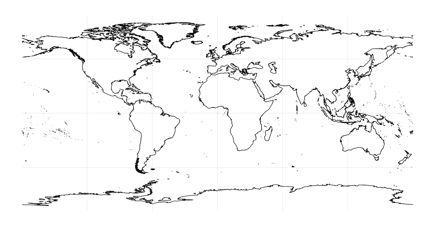
world_coastline
Visit Britain
Let’s narrow our focus on just Great Britain, which we can do by clipping the limits of the plot to a bounding box with a southwestern corner of 49.7º N 10.6º W and a northeastern corner of 60.85ºN 1.9ºE6.
ggplot() +
    geom_sf(data = world_coastline) +
    xlim(-10.6, 1.9) +
    ylim(49.7,60.85)
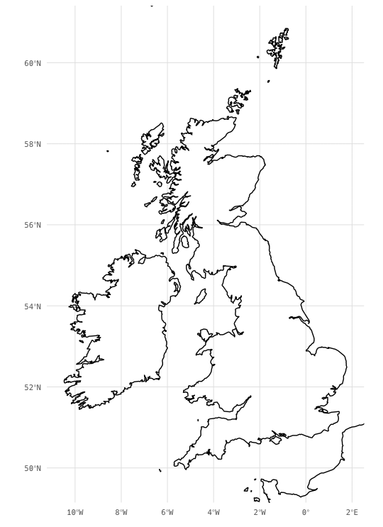
world_coastline zoomed in on Great Britain
So we can zoom in on the coastline, great, but at the moment it’s still part of the world_coastline object, and if we look back at the summary of that object besides the geometry column that contains the spatial data there’s no defining information that can help us pick out Great Britain from the other objects.
This is where using {sf} again helps us, as the simple features standard includes all sorts of conventions for interrogating and transforming geospatial data.
Firstly let’s define a reference point that we know is in Great Britain. So how about the point that all distances from London are measured7, a point known as kilometre zero in mapping circles. We can do this by creating a tibble with the reference point, and then converting it to an {sf} object using sf::st_as_sf(). When converting raw longitude and latitude data we also need to tell {sf} what coordinate reference system (CRS) we’re using. The number 4326 corresponds to the WGS84 projection system, which is what our existing world_coastline object is using (see the datum reference in the summary of the object listed above). We can also confirm this by adding the point to our plot.
gb_ref_point <- tibble::tribble(
  ~point,   ~longitude, ~latitude
  "London",   -0.12768,  51.50739
  ) %>%
  sf::st_as_sf(coords = c("longitude", "latitude"), crs = 4326)

ggplot() +
    geom_sf(data = world_coastline) +
    geom_sf(data = gb_ref_point, colour = "red") +
    xlim(-10.6, 1.9) +
    ylim(49.7,60.85)
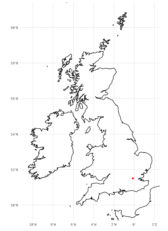
London’s kilometre zero
Finding Londo8
We can now use another handy {sf} function to find the shape in world_coastline that our Great Britain reference point sits within. However, first we need to convert our coastline into shapes. “Hang on” I hear you cry, isn’t it already a set of shapes? To our eyes yes; but to R it’s not, it’s a set of lines, or what {sf} calls a LINESTRING which is a set of points that form a line. The first and last point in each shape’s linestring that we see is the same set of coordinates. So at present each shape is just a line that while ending in the same place isn’t actually defined as an enclosed shape, or in vector terminology a polygon. But thankfully {sf} will easily allow us to convert these linestrings to polygons. From there we can then use another {sf} function to find which polygon contains our reference point. With a bit of trial and error I found that I could use sf::st_within() to do this matching and then use that as a way to subset my original world_coastline object to get a gb_coastline.
gb_coastline <- world_coastline[as.numeric(sf::st_within(gb_ref_point, world_polygons)),]

ggplot() +
    geom_sf(data = world_coastline, colour = "grey60") +
    geom_sf(data = gb_coastline, colour = "blue") +
    geom_sf(data = gb_ref_point, colour = "red") +
    xlim(-10.6, 1.9) +
    ylim(49.7,60.85)
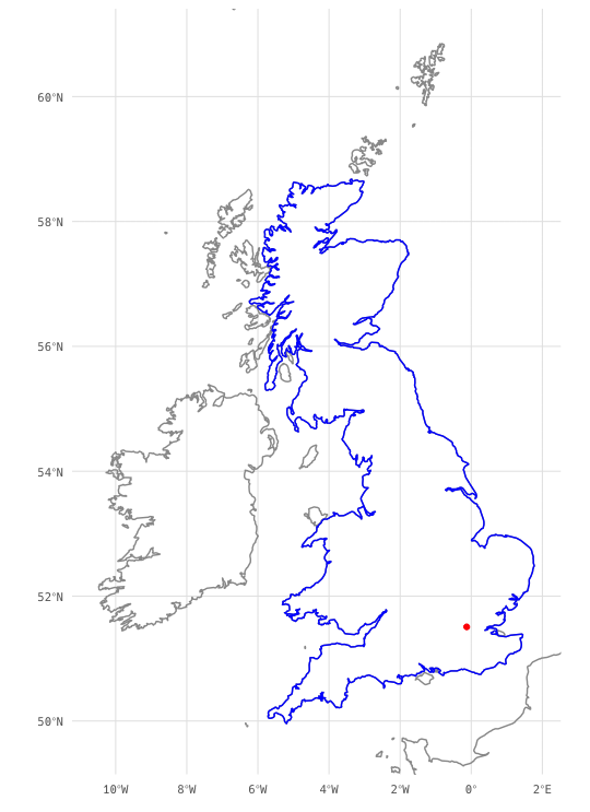
gb_coastline
And lo, we’ve now got an object representing the coastline of Great Britain.
One small step for our mapbot, one giant leap for mapbotkind
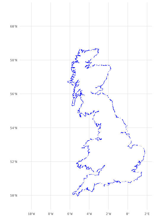
Now that we’ve got our gb_coastline object we can inspect it a bit further. Firstly, we can extract the points from the linestring, which tells us that the line drawn in the Natural Earth data that creates the shape of Great Britain consists of 3,707 points. This also creates a plot, evoking the style of pointillist art, showing some areas with a high density of points such as the sea lochs of western Scotland and a few areas with a very low density of points such as the north Norfolk and north Kent coasts.
gb_coast_points <- sf::st_cast(gb_coastline, "POINT")
gb_coast_polygon <- sf::st_polygonize(gb_coastline)

ggplot() +
    geom_sf(data = gb_coast_polygon, fill = "white", colour = NA) +
    geom_sf(data = gb_coast_points, colour = "blue", shape = ".") +
    xlim(-10.6, 1.9) +
    ylim(49.7,60.85) + mattR::theme_lpsdgeog()
> str(gb_coast_points)

Classes ‘sf’ and 'data.frame':	3707 obs. of  4 variables:
 $ featurecla: chr  "Coastline" "Coastline" "Coastline" "Coastline" ...
 $ scalerank : chr  "0" "0" "0" "0" ...
 $ min_zoom  : num  0 0 0 0 0 0 0 0 0 0 ...
 $ geometry  :sfc_POINT of length 3707; first list element:  'XY' num  -3.32 56.37
 - attr(*, "sf_column")= chr "geometry"
 - attr(*, "agr")= Factor w/ 3 levels "constant","aggregate",..: NA NA NA
  ..- attr(*, "names")= chr [1:3] "featurecla" "scalerank" "min_zoom"
gb_coast_points
Let’s use our gb_coast_points object to take a couple of initial steps.
> gb_coast_points$geometry[1:3]

POINT (-3.323476 56.36591)
POINT (-3.311513 56.35651)
POINT (-3.294016 56.35277)
Now let’s go a bit further and plot our first 10 steps.
ggplot() +
    geom_sf(data = gb_coastline, colour = "grey80", size = 1) +
    geom_sf(data = gb_coast_points[1:10,], colour = "blue", size = 4) +
    xlim(-3.4, -2.8) +
    ylim(56.3, 56.5)
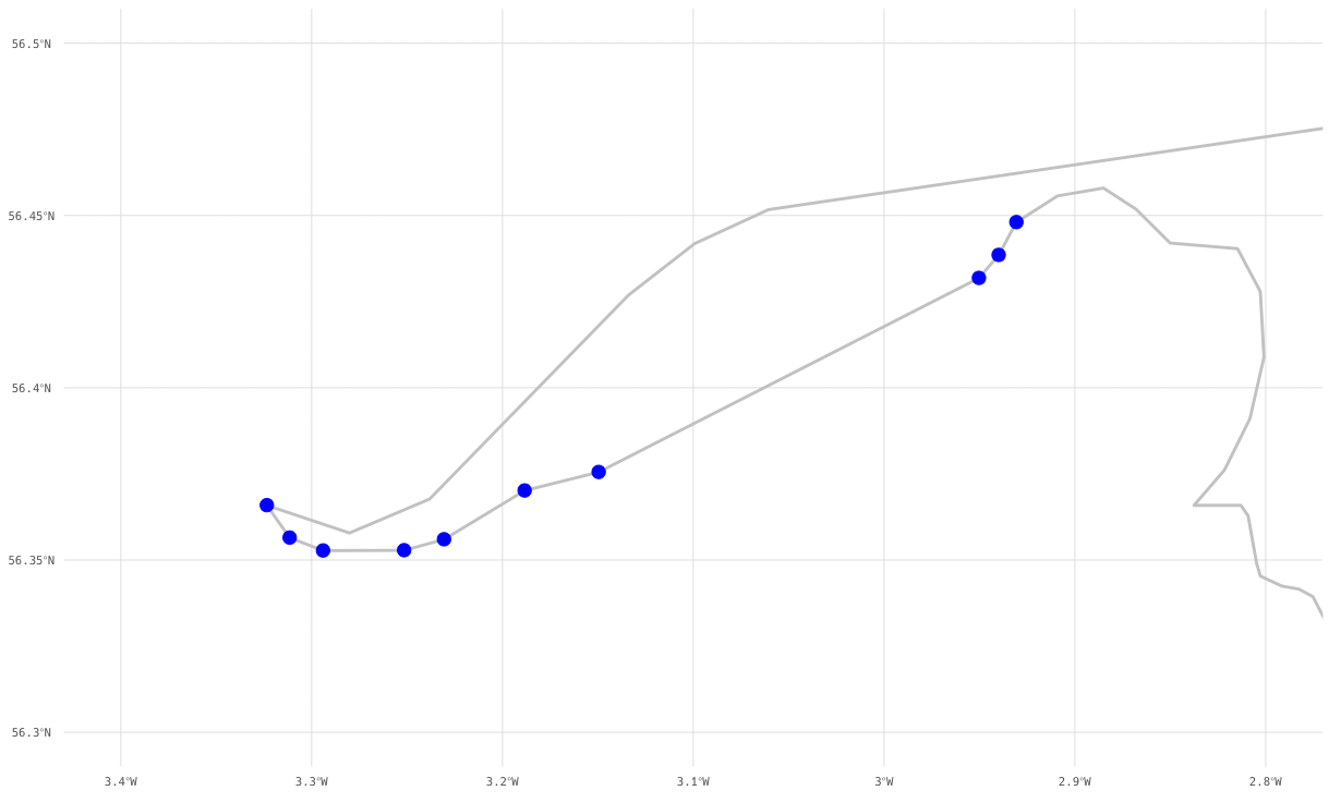
The first 10 points in the gb_coast_points object
If we look at Open Street Map we can find out where this is in the real world, rather than just a set of points on a plot. It turns out this is a walk from the mouth of the river Tay (by the hamlet of Inchyra, southeast of Perth) along its firth to Newport-on-Tay opposite Dundee.
It turns out that these first 10 steps weren’t that short a walk, as the crow flies it’s around 26 kilometres. Is this ok for a bot, or should the bot simulate a more human experience of walking along the coast. If the latter then we might want to use a more higher resolution set of coastline data, but more on that another time.
-
Copyright to Matt Dray… he’s very jealous of the tidyverse (nee Hadleyverse) and wants his own. ↩︎
-
The londonmapbot, the canberramapbot and the narrowbotr. ↩︎
-
That is until coastal erosion redefines it. ↩︎
-
Greenland is the world’s largest island, and Wikipedia lists a further 321 islands of more 1,000 km^2^. Let’s maybe not get into the definition of an island, unless you want to talk about islands in lakes on islands in lakes. Natural Earth’s definitions don’t actually make clear what is included in their main coastline data or their minor islands dataset. Suffice to say, Great Britain is a sufficiently large island to be included in the main coastline data (phew). ↩︎
-
This is actually a bounding box that contains all the most northern, southern and eastern points of the United Kingdom (including the Isles of Scilly) and the westernmost point of Ireland. Technically, Rockall is the westernmost point in the United Kingdom but it’s literally just a rock (hence the name). Because of the way
ggplot2::geom_sf()crops map data this specific plot also appears to capture almost all of the Channel Islands (all the inhabited places, but their southernmost point is a reef that I think is roughly where the top of the 2ºW is rendered as an axis label). ↩︎ -
Reader, determining the exact position (51.50739ºN 0.12768ºW) was actually surprisingly difficult. Common knowledge is that the measurement is taken from Charing Cross. But not it’s not the railway station or the cross that sits outside it, rather it is the site of the original Eleanor Cross (the one outside Charing Cross station being a replica), the position of which is marked by a plaque next to the statue of King Charles I on the roundabout south of Trafalgar Square (sidenote: is it not a bit weird we still have a statue in the dead centre of London of the King we beheaded, no?). However, I could not find anywhere that specifically documented the coordinates of such an important location — many a Google search will tell you about the plaque but none tell you the specific location, and the only reference to an Ordnance Survey source I could find was to content that has since disappeared. Even trying to use Google Maps and finding the plaque on its satellite imagery resulted in a set of coordinates that did not when trying them independently render a marker on the plaque. OpenStreetMap is our hero, there is a marker for the plaque that is separate from the statue, and centring the map on that point gives rise to our coordinates (if we inspect the map URL that is). ↩︎
-
Not a typo, but Finding Nemo pun, I’m dead funny me. ↩︎