gongoozler [n] a person who enjoys watching boats and activities on canals
I’m sure I’m not the first person, and won’t be the last, to remark that 2020 is a very strange year. October 2020 marks five years since I last went on a canal boat holiday. An anniversary that at the outset of this year I had hoped I might have managed to avoid by taking to the water sometime over the summer. So, inspired by Matt Dray’s recent adventures in location-based Twitter-botting, I wondered whether it might be possible to make a Twitter bot that showcased features of the British canal network. So let me introduce you to narrowbotR … see what I did there, an R based twitter bot that does things narrowboats do.
How it works
Based on the principles of Matt’s londonmapbot, narrowbotR uses Github Actions to do the following:
- Select a random location on the English and Welsh canal network
- Get a photo for the location
- Post a tweet
Matt’s bot is a lightweight bot that picks a random location within an effective bounding-box (by selecting random numbers between the east-west and north-south extents), grabs an image from the Mapbox API, and then constructs and posts a tweet via the {rtweet} package which includes a link to the location in OpenStreetMap. This process is encapsulated in a single script, which is then executed every 30 minutes by a Githhub Action YAML workflow.
narrowbotR extends the programming in a number of ways:
- It builds and samples a dataset of geospatial features on the canal network.
- It access the Flickr API as well as the MapBox API.
- It constructs a rich status message and posts this via a customised version of the
rtweet::post_tweet()function to embed the location in the tweet’s metadata. - The GitHub Action operates only between 7am and 9pm because responsible boaters don’t cruise after night.
Matt’s bot runs from a single script, but in order to do all of the above narrowbotR is a collection of functions and a runner. The repo’s structure is also follows:
narrowbotR
  │
  ├ .github/workflows
  │  ├ R_check.yaml.       # A manual workflow to check R on Github Actions
  │  ├ bot.yaml.           # The workflow controlling the scheduled bot
  │  └ bot_manual.yaml     # The bot workflow but with manual execution
  │
  ├ data
  │  ├ all_points.RDS      # A dataset of all the CRT point data
  │  ├ features.csv        # Metadata about types of CRT features
  │  └ feeds.csv           # URLs to the feeds for CRT geodata
  │
  ├ R
  │  ├ build_database.R    # A script to build data/all_points.RDS
  │  ├ flickr_functions.R  # Functions to interact with the Flickr API
  │  ├ pkg_install.R       # Functions to install packages on Github Actions
  │  └ post_geo.R          # A function to extent rtweet::post_tweet
  │
  ├ LICENCE                # An MIT licence for the code
  ├ narrowbot.R            # The bot workflow script
  └ README.md              # The repo README
bot.yaml runs the bot to a schedule and calls narrowbot.R to do the legwork, I’ll discuss these towards the end of the blog, first I’ll run through the main steps: building a database, accessing the Flickr API, and posting a geo-aware tweet.
Building a database
As Ken Butler points out, londonmapbot benefits from the fact that London occupies a relatively rectangular space that is relatively neatly aligned against the east-west and north-south axes of most coordinate systems. Matt helps this by saying that londonmapbot’s parameters are to find locations within the M25 which is rather more rectangular than the boundary of the Greater London region.
The UK’s inland waterways system doesn’t exist in such a neat set of geographical parameters, moreover it doesn’t exist as a single system. There are three major navigation authorities — the Canal and River Trust (for England and Wales, and itself a relatively recent merger formed of British Waterways and part of the Environment Agency), Scottish Canals (for Scotland), and Waterways Ireland (covering both Northern Ireland and the Republic of Ireland). But there also exist separate navigation authorities for specific watercourses/sets of waterways that aren’t covered by these bodies, the largest of these being the Broads Authority in Norfolk. To keep things simple, at the moment I’ve limited narrowbotR to working within the confines of the Canal and River Trust (CRT) network.
Thankfully, CRT publish a large amount of open geodata about their network, which made the process of building a database fairly easy. Different types of feature exist in their own GeoJSON feed, but it was fairly simple enough to create a simple csv listing these feeds, and then using {purrr} to run through these, download the data and combine it.
feeds <- readr::read_csv("data/feeds.csv")

points <- feeds %>%
  dplyr::filter(geo_type == "point") %>%
  dplyr::mutate(data = purrr::map(feed_url, sf::st_read))
We also need to clean the file a little:
- the data includes points, polygons and lines, at this stage let’s just concern ourselves with the point data;
- some features include an angle but this is stored in variables with different capitalisation, so let’s unify that;
- let’s extract the latitude and longitude positions of the point from the geometry;
- let’s add some metadata about the features that we’ve created in a separate csv;
- finally, let’s rename some of the fields to give them a slightly clearer name.
features <- readr::read_csv("data/features.csv")

points_combined <- points %>%
  tidyr::unnest(data) %>%
  dplyr::mutate(angle = dplyr::case_when(
    !is.na(Angle) ~ as.double(Angle),
    !is.na(ANGLE) ~ as.double(ANGLE),
    TRUE ~ NA_real_
  )) %>%
  bind_cols(sf::st_coordinates(.$geometry) %>%
              tibble::as_tibble() %>%
              purrr::set_names(c("long", "lat"))) %>%
  dplyr::left_join(features, by = c("feature", "SAP_OBJECT_TYPE")) %>%
  dplyr::select(-Angle, -ANGLE, -OBJECTID) %>%
  janitor::clean_names() %>%
  dplyr::rename(uid = sap_func_loc,
         name = sap_description,
         obj_type = sap_object_type)

readr::write_rds(points_combined,"data/all_points.RDS", compress = "bz2")
At present this dataset is created by manually running this script. We could create this every time narrowbotR but that is definite processing overkill as the data doesn’t appear to be updated that regularly. In future I plan to write a script and Github Action to check on an occasional interval whether any of the CRT feeds have been updated and at that point issue a call to rebuild the dataset.
Selecting a Flickr photo
londonmapbot pulls an aerial photograph from the Mapbox API, but sometimes canal features are difficult to identify from above and/or can be things of interest to photographers. Flickr is an online photo sharing service, yes younglings we were able to share photos before Instagram, and has an API that allows you to access photos shared on the service. Photographers are able to geotag their photos, and using the Flickr API we’re able to search for photos based on their location. There are some packages that have tried to provide access in R to the Flickr API but they aren’t well maintained. Thankfully for the work narrowbotR does there’s no need for a complex OAuth authentication proccess and the standard API access key is all that’s needed. To get a Flickr API key you just need to sign up to create an app.
Getting Flickr photos
To get the photos for a location we’ll use the flickr.photos.search API, let’s create the flickr_get_photo_list() function to handle this.
flickr_get_photo_list <- function(key = NULL, lat, long) {

  if (is.null(key)) {
    key <- Sys.getenv("FLICKR_API_KEY")
    if (key == "") {
      stop("Flickr API key not set")
    }
  }

  if (missing(lat)) {
    stop("lat missing")
  }

  if (missing(long)) {
    stop("long missing")
  }

  # construct flickr api url
  # using lat/long will sort in geographical proximity
  # choose within 100m of the position (radius=0.1)
  url <- paste0(
    "https://www.flickr.com/services/rest/?method=flickr.photos.search",
    "&api_key=", key,
    "&license=1%2C2%2C3%2C4%2C5%2C6%2C7%2C8%2C9%2C10",
    "&privacy_filter=1",
    "&safe_search=1",
    "&content_type=1",
    "&media=photos",
    "&lat=", lat,
    "&lon=", long,
    "&radius=0.1",
    "&per_page=100",
    "&page=1",
    "&format=json",
    "&nojsoncallback=1"
  )

  # get data
  r <- jsonlite::fromJSON(url)

  # extract the photo data
  p <- r$photos$photo

  ...

 }
First the function will check if an API key is provided and if not it’ll look and see if its been set as an environment variable, if no key is available the function will throw an error. Similarly if no lat or long are provided let’s throw an error. To avoid this error during testing we could put in place some limits for the lat and long to check they’re within the extent of the UK but let’s not overcomplicate, and make it easy for folk to port the code.
Next let’s construct our call to the flickr.photos.search API - this is in the format of a URL string with a series of arguments. We must supply the api.key argument, in addition to the lat and lon arguments, let’s refine the call a bit further. The licence argument selects only those photos that are licenced for re-use. We also set the privacy_filter and safe_search to make sure we select photos suitable for broad public consumption. The content_type and media arguments ensure we just get photos, not screenshots or videos. In addition to the lat and lon arguments we can also set a radius (in km) from the point, in this case we’re only going to ask for photos within 100m (0.1km) of the location; when lat and lon are specified the search will return photos in ascending order of proximity to the location (i.e. the first result will be the closest to the specified point). In the event of picking a very popular location, the per_page and page arguments ensure we only get the first 100 photos. Finally the format and nojsoncallback arguments are required for getting the data in JSON format.
Now we’ve constructed our URL we can get the data by calling on jsonlite::fromJSON(), which returns a list object within which there is a table of the photo data that we can extract.
Let’s continue building our function by working with this table (the object p).
flickr_get_photo_list <- function(key = NULL, lat, long) {

  ...

  # skip if less than 10 photos returned
  # suggests uninteresting/remote place
  if (length(p) == 0) {
    p <- NULL
  } else if (nrow(p) < 10) {
    p <- NULL
  } else {

    # get info for photos, add sunlight hours
    # drop photos before sunrise or after sunset
    p <- p %>%
      dplyr::mutate(
        info = purrr::map2(id, secret,
                           ~flickr_get_photo_info(key = key,
                                                  photo_id = .x,
                                                  photo_secret = .y))
      ) %>%
      tidyr::unnest(info) %>%
      dplyr::mutate(
        suntimes = purrr::map(
          as.Date(date),
          ~suncalc::getSunlightTimes(date = .x, lat = lat, lon = long,
                                     keep = c("sunrise", "goldenHourEnd",
                                              "goldenHour", "sunset"))),
        suntimes = purrr::map(suntimes, ~dplyr::select(.x, -date, -lat, -lon))
      ) %>%
      tidyr::unnest(suntimes) %>%
      dplyr::mutate(after_sunset = date > sunset,
                    before_sunrise = date < sunrise,
                    goldenhour = dplyr::if_else(
                      (date >= sunrise & date <= goldenHourEnd) |
                        (date <= sunset & date >= goldenHour), TRUE, FALSE)) %>%
      dplyr::filter(!after_sunset) %>%
      dplyr::filter(!before_sunrise)

    # if after removing night-time photos there are only a very small number
    # then exclude again as might be an uninteresting place
    if (nrow(p) < 3) {
      p <- NULL
    }

  }

  return(p)

}
If there are less than 10 photos we’ve probably selected somewhere fairly remote and/or uninteresting. In one of my first tests was a hidden culvert for a sewer that was close to a Morrisons’ car park which returned only three photos all of which were of the car park, which is just what we want, isn’t it (it’s not). So when there are no/a small number of photos then let’s just set p to NULL and be done with it. But if we get more than 10 photos let’s get some more data about the photos, using another custom function (flickr_get_photo_info, of which more in a second) this will give us information including the date and time the photo was taken. Using the date as well as the latitude and longitude of the position we can use the {suncalc} package to identify sunrise and sunset times for the location and exclude photos taken at night, we can also calculate if the photo was taken during “golden hour” which is a prime time for photography.
The flickr_get_photo_info() function accesses the flickr.photos.getInfo API to access further data about specific photos using the photo_id and photo_secret data returned by our call to the search API.
flickr_get_photo_info <- function(key = NULL, photo_id, photo_secret) {

  if (is.null(key)) {
    key <- Sys.getenv("FLICKR_API_KEY")
    if (key == "") {
      stop("Flickr API key not set")
    }
  }

  if (missing(photo_id)) {
    stop("photo_id missing")
  }

  if (missing(photo_secret)) {
    stop("photo_secret missing")
  }

  # create flickr api url
  url <- paste0(
    "https://www.flickr.com/services/rest/?method=flickr.photos.getInfo",
    "&api_key=", key,
    "&photo_id=", photo_id,
    "&secret=", photo_secret,
    "&format=json",
    "&nojsoncallback=1")

  # get data
  r <- jsonlite::fromJSON(url)

  # extract relevant info
  info <- tibble::tibble(
    username = r$photo$owner$username,
    realname = r$photo$owner$realname,
    licence = r$photo$license,
    description = r$photo$description$`_content`,
    date = lubridate::as_datetime(r$photo$dates$taken),
    can_download = r$photo$usage$candownload,
    can_share = r$photo$usage$canshare
  )

  return(info)

}
As with the flickr_get_photo_list() function, we’ll check for an API key and that the other arguments aren’t missing. Our API call this time is much smaller, needing just the api_key, photo_id and secret to get a dataset returned to us. We don’t need all the data provided, so let’s build a small tibble of the data we might need: details about the photographer, the licence, the caption/description, the data, and whether the photo can be downloaded/shared.
Scoring photos
flickr_photos_list() returns either a NULL value or a tibble of up to 100 photos selected from Flickr. How should we select a photo? We could just take the first item in the list, which according to the Flickr API documentation is the closest to the feature. But as I discovered during my testing, sometimes this isn’t a particularly interesting photo or one related to the canal network. When testing, one location I had randomly selected was a site in central Birmingham that happened to be close to some of the HS2 construction work, and so the closest photo to the position selected was actually of this. There might also be issues with Flickr users correctly geo-positioning their photos, many modern cameras automatically embed this information, but you can manually place your photos on a map within the Flickr UI.
So why not build a scoring algorithm to try and pick a “good” photo. Flickr has its own internal algorithm called “interestingness”, but it’s not published so we don’t know how Flickr rates interestingness, plus it’s no fun using someone else’s algorithm is it. And lo the function flickr_photo_score() is born.
flickr_photo_score <- function(df) {

  n_df <- df %>%
    dplyr::select(id, owner, title, description, date, goldenhour) %>%
    dplyr::mutate(
      title_words = purrr::map_dbl(title, ~max(stringr::str_count(., " "),1)),
      desc_words = stringr::str_count(description, " "),
      total_words = title_words + desc_words,
      desc_words2 = log10(purrr::map_dbl(description, ~max(stringr::str_count(., " "),1))),
      word_score = purrr::pmap_dbl(list(title_words, desc_words2), sum, na.rm = TRUE),
      canal_words = canal_word_count(title) + canal_word_count(description),
      canal_word_score = purrr::map_dbl(canal_words^2, ~max(., 1)),
      gold = dplyr::if_else(goldenhour, 2, 1),
      offset = Sys.time() - date
      ) %>%
    dplyr::filter(offset <= 5000) %>%
    dplyr::mutate(
      distance = dplyr::row_number(),
      dist_rev = rev(sqrt(distance))
    ) %>%
    dplyr::arrange(offset) %>%
    dplyr::mutate(
      offset_rev = rev(sqrt(as.numeric(offset))),
      alt_off = rescale(as.numeric(offset), c(5,1)),
      final_score = word_score * dist_rev * gold * alt_off * canal_word_score
      ) %>%
    dplyr::select(id, owner, final_score) %>%
    dplyr::arrange(-final_score)

  return(n_df)

}
Our scoring function takes the tibble produced at the end of flickr_get_photo_list() and makes some calculations based off the metadata, which will then power the scoring. So what shall we use in our scoring?
Words
There are two fields that Flickr users can use to describe their photos: the title and the description. Let’s do some analysis of these to get some metrics about the words used to describe the photo. Longer titles probably mean someone has taken time to label their work rather than use the filename, so we get a word count of the title in title_words. A longer descriptions is probably also an indicator that someone has taken the time to write about their photo, as it turns out some people write a lot and we perhaps don’t want to reward the overly verbose so actually let’s get the log10() of the number of words in the description, this is stored as desc_words2 (desc_words being the simple word count). Let’s then sum total_words and desc_words2 to get an overall word_score.
But thinking back to my HS2 photo issue in Birmingham, is there a way to prioritise canal-related words? Of course, let’s write a canal_word_count() function to do this.
canal_word_count <- function(string) {

  canal_words <- c("canal", "lock", "water", "boat", "gate", "bird", "duck",
                   "swan", "river", "aqueduct", "towpath", "barge", "keeper",
                   "tunnel", "narrow")

  counter <- 0

  for (word in canal_words) {
    x <- stringr::str_detect(tolower(string), word)
    counter <- counter + x
  }

  return(counter)

}
canal_word_count() takes a string and compares it to a list of canal-related words. Specifically let’s look for the words: canal, lock, water, boat, gate, bird, duck, swan, river, aqueduct, towpath, barge, keeper, tunnel and narrow. We iterate over the list of these words and detect whether they’re in use. By using stringr::str_detect() over string::str_count() we prefer those who are using multiple canal-related words rather than just using a single word lots of times. Again, a decision influence by that HS2 construction near New Canal Street in Birmingham.
In our selection algorithm we count the number of canal-related words used in the title and description, and sum these. Then to give it even more power let’s square the result to come up with our canal_words_score.
Time and date
In flickr_get_photo_list() we get a TRUE/FALSE marker for whether the photo was taken during golden hour, R’s will naturally interpret TRUE as 1 and FALSE as 0, we don’t want any photo outside of golden hour to get a 0, so let’s set gold as 2 for TRUE and 1 for FALSE.
Let’s also calculate recency, we can do this by subtracting the date-time of the photo from the current time provided by Sys.time(), which we’ll call offset. Let’s prefer ‘recent’ photos and drop any photos that are older than 5,000 days which gives us photos from around 2008 onwards (though maybe I’ll remove this condition in future). The code still includes lines from experiments with reversing the offset, but the algorithm uses a rescaled version of the offset where the smallest offset is given a value of 5 and the largest offset is given a value of 1.
Distance
The Flickr API doesn’t give us the actual distance, but the documentation claims that search results for geo-based searches are returning in ascending distance from the search location. Therefore we can use the row ordering as a proxy for distance, and we set distance to this using dplyr::row_number(), we can then reverse the order using base::rev() so that the first row gets the number of the last row (i.e. the largest number). As we set a relatively tight radius for the photo let’s not over penalise photos, especially in popular places, so in calculating dist_rev let’s take the square root of our proxy distance.
Scoring the photos
Finally, we can now calculate a score, let’s just calculate this as a product of our different components: final_score = word_score * dist_rev * gold * alt_off * canal_word_score. We can then return a dataset of the scores.
Picking a photo
Picking a photo is done by the flickr_pick_photo() function. This function calls the scoring function we just wrote, so it also takes as it’s argument the tibble created by flickr_get_photo_list().
flickr_pick_photo <- function(df) {

  scored_df <- flickr_photo_score(df)

  n_df <- df %>%
    dplyr::inner_join(scored_df, by = c("id", "owner")) %>%
    tidyr::drop_na(final_score) %>%
    dplyr::filter(final_score == max(final_score))

  photo <- as.list(n_df)

  photo$photo_url <- paste("https://www.flickr.com/photos",
                           photo$owner,
                           photo$id,
                           sep = "/")

  photo$img_url <- paste0("https://live.staticflickr.com/",
                         photo$server, "/",
                         photo$id,"_",photo$secret,".jpg")

  return(photo)

}
First, we get the scores for the dataset using flickr_photo_score(), let’s then merge these scores with the original dataset, let’s remove anything that might have a missing score for some reason, and then let’s select the observation with the highest score.
As we’re only selecting one item, let’s convert this to a list to make it a little bit easier to work with, which we can easily do with base::as.list(). Let’s then append to this list two URLs from Flickr which can be built from the data we already have in our list: (i) the URL of the Flickr webpage for the photo, and (ii) the URL of the actual image file so that we can download the photo.
And voila, if we’re lucky we’ve now got the information we need to get an image from Flickr for our tweet.
Posting a geo-tweet
londonmapbot makes use of the {rtweet} package’s post_tweet() function. This provides an easy way to post tweets from within R via the Twitter developer API, including media objects (e.g. images).
The Twitter API allows you to also embed location details in your tweet, which Twitter will then use this to connect the tweet to the nearest locality. rtweet::post_tweet() does not support this functionality. So narrowbotR extends this by creating a post_geo_tweet() function. Most of the code for post_geo_tweet() is taken directly from the source code for rtweet::post_tweet(). In fact there are only three lines that have been added.
if (!is.null(lat) & !is.null(long)) {
    params <- append(params, list(lat = lat, long = long, display_coordinates = TRUE))
  }
Here we’re adding (if they’re provided) the latitude and longitude as parameters to the param object that will be passed to the rtweet::make_url() function that constructs Twitter API calls.
Cruising the canals
Now that we’ve built all of our functionality we can create the narrowbot.R script that will cruise the canals, select an object and post a tweet. First let’s get set-up
# load functions
library(dplyr)
source("R/post_geo_tweet.R")
source("R/flickr_functions.R")

message("Stage: functions loaded")

# create twitter token
narrowbotr_token <- rtweet::create_token(
  app = "narrowbotr",
  consumer_key =    Sys.getenv("TWITTER_CONSUMER_API_KEY"),
  consumer_secret = Sys.getenv("TWITTER_CONSUMER_API_SECRET"),
  access_token =    Sys.getenv("TWITTER_ACCESS_TOKEN"),
  access_secret =   Sys.getenv("TWITTER_ACCESS_TOKEN_SECRET")
)

message("Stage: Twitter token created")
Let’s load {dplyr} so that we can use the pipe (%>%) and then source our custom functions. We also need to create a token for working with Twitter, which we can do through rtweet::create_token() and our Twitter Developer API keys/tokens. We’re also providing message() calls periodically so that when it runs in Github Actions the script is “chatty” and provides some messages that we can see in the Action’s log file so that we can more easily diagnose issues/review what has happened.
Let’s then get the points dataset, the geometry column is includes data in a format controlled by {sf}, we don’t need to install or load {sf} for the bot, so in order to easily interact with the dataset let’s drop this column. Culverts are generally pipes/passages that direct watercourses under something and often hidden from public view so let’s filter these out of the dataset. Finally let’s pick one item at random and then convert the tibble to a list.
In our message at this point, let’s announce the place that was selected - this can be particularly helpful for diagnosing problems.
# load points data
all_points <- readRDS("data/all_points.RDS")

# pick a point
place <- all_points %>%
  dplyr::select(-geometry) %>%
  dplyr::filter(stringr::str_detect(feature, "culvert", negate = TRUE)) %>%
  dplyr::sample_n(1) %>%
  as.list()

message("Stage: Picked a place [", place$name,
        ", lat: ", place$lat,
        ", long: ", place$long, "]")
Now we’ve selected a place let’s see if we can get a Flickr photo for it.
place_photos <- flickr_get_photo_list(lat = place$lat, long = place$long)

message("Stage: Got photos")

if (is.null(place_photos)) {
  photo_select <- NULL
  message("Stage: No photo selected\n")
} else {
  photo_select <- flickr_pick_photo(place_photos)
  message("Stage: Photo selected\n")
}
We get the photos through a call to our trusty flickr_get_photo_list() function, if we get a NULL response then let’s also record our photo_select object as NULL. If we have got a list of photos let’s pick a photo. Now we’ve selected a photo we can download it, but what if we don’t have a Flickr photo? Let’s revert to the example of londonmapbot an use an aerial photo from Mapbox.
tmp_file <- tempfile()

if (is.null(photo_select)) {
  img_url <- paste0(
    "https://api.mapbox.com/styles/v1/mapbox/satellite-v9/static/",
    paste0(place$long, ",", place$lat, ",", 16),
    "/600x400?access_token=",
    Sys.getenv("MAPBOX_PAT")
  )
} else {
  img_url <- photo_select$img_url
}

download.file(img_url, tmp_file)

message("Stage: Photo downloaded")
We’re not going to need to store our downloads after we’ve posted it so let’s put it in a temporary file by calling tempfile(). If our photo_select is NULL we construct a simple call to the Mapbox API for satellite imagery, and we’ll zoom in a bit closer than londonmapbot as canal features might be difficult to ascertain unless we’re zoomed in at a good distance. If photo_select isn’t NULL remember that in picking a photo we added two URLs to the photo’s list object, let’s grab the URL for the image. Now that we have a URL for an image from either Mpabox or Flickr we can download the image.
We’ve now got all the pieces we need to construct a tweet.
base_message <- c(
  "📍: ", place$name, "\n",
  "ℹ️: ", place$obj_type_label, "\n",
  "🗺: ",  paste0("https://www.openstreetmap.org/",
                  "?mlat=", place$lat,
                  "&mlon=", place$long,
                  "#map=17/", place$lat, "/", place$long)
)

if (is.null(photo_select)) {
  tweet_text <- base_message
} else {
  tweet_text <- c(
    base_message, "\n",
    "📸: Photo by ", stringr::str_squish(photo_select$realname), " on Flickr ",
    photo_select$photo_url)
}

status_msg <- paste0(tweet_text, collapse = "")

message("Stage: Tweet written")
Let’s start with the first part of our tweet which will always be the same: the name of the place, the type of place, and a link to the location in OpenStreetMap. We’ll use emoji to provide a key for these three pieces of information. If we’ve got a Flickr photo let’s also add details about the photo by saying who the photographer is and providing the URL to the Flickr webpage for the photo.
Our twitter messages so far are R character vectors with multiple items, we need to use base::paste0() to merge all of the items into a single character string.
We then post our tweet using post_geo_tweet(). And let’s also print the tweet for the Github Actions log.
post_geo_tweet(
  status = status_msg,
  media = tmp_file,
  lat = place$lat,
  long = place$long
  )

message("Stage: Action complete")

message("\n====\nTweet:\n")

cat(status_msg)
Cruising all day, moor up at night
Finally, let’s create a Github Action workflow so that our narrowbot.R can “cast off” and cruise the canals through the day. Historically the canals operated 24/7, but an important rule of modern canal boating “no cruising after dark”, this is to ensure you don’t disturb moored boats and most canals and boats do not have good lighting so you may well get yourself into trouble.
In my post on automating PDF scraping I talked about my first use of Github Actions. I’ve not done much more since, and the principles are similar. However, since that earlier work if you use Github’s MacOS runner then R comes already built, and so there’s no longer a need to include installation of R as part of your action workflow.
name: narrowbotR

on:
  schedule:
    - cron:  '10,40 7-20 * * *'

jobs:
  narrowbotR-post:
    runs-on: macos-latest
    env:
      FLICKR_API_KEY: ${{ secrets.FLICKR_API_KEY }}
      TWITTER_CONSUMER_API_KEY: ${{ secrets.TWITTER_CONSUMER_API_KEY }}
      TWITTER_CONSUMER_API_SECRET: ${{ secrets.TWITTER_CONSUMER_API_SECRET }}
      TWITTER_ACCESS_TOKEN: ${{ secrets.TWITTER_ACCESS_TOKEN }}
      TWITTER_ACCESS_TOKEN_SECRET: ${{ secrets.TWITTER_ACCESS_TOKEN_SECRET }}
      MAPBOX_PAT: ${{ secrets.MAPBOX_PAT }}

    steps:
      - uses: actions/checkout@v2
      - name: Install packages
        run: Rscript -e 'source("R/pkg_install.R")' -e 'install_runner_packages()'
      - name: Cruise the canals
        run: Rscript narrowbot.R
Let’s set a cron schedule to 10,40 7-20 * * * which crontab.guru tells us is the syntax for running the worklow “at minute 10 and 40 past every hour from 7 through 20”. Github Actions scheduler works on UTC all-year round so this means we’ll get two tweets an hour between 7am-8pm during the winter and 8am-9pm during the summer, as the workflow will take a couple of minutes to set-up and run, this should mean that tweets are posted at roughly quarter-past and quarter-to the hour.
Having set a schedule, let’s use Action Secrets to store and get the various API keys and tokens we need.
Now let’s run our R scripts, first off let’s install the packages needed to run the script. We do this by sourcing the pkg_install.R script and then running the install_runner_packages() function. When building the dataset I said that in due course I’ll write a function to automate checking and building the database which will require additional packages, notably {sf}. Having installed the required packages we can now dispatch our narrowboater and let them find a feature and tweet about it by running the narrowbot.R script.
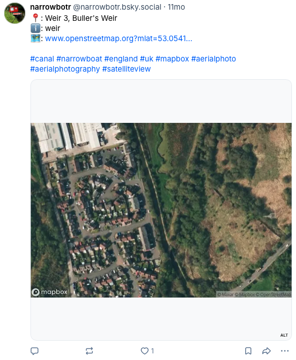
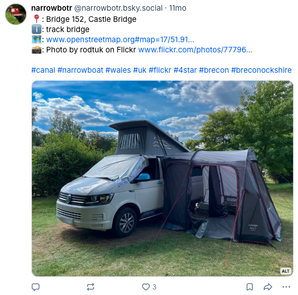
And voila, we have ourselves Twitter bot of the Canal and River Trust network. Why not give it a follow, and get tweets like the following.
See below for examples of the bot’s posts. Owing to the deactivation of the bot’s Twitter account in 2025 these have been taken from its Bluesky account.