The interplanetary birthday express

Hello Humans, we cake in peace. We here at the Interplanetary Cake Union have noticed that you are missing out on the opportunity of celebrating your birthday more often by not knowing about your birthdays on other planets, and thus are potentially depriving yourself of more cake eating opportunities. Please use our birthday planets tool to review your age on other planets in the solar system, when your next birthday is and then use our Interplanetary Birthday Express service to order yourself a galactic collection of cake¹.

TLDR: I’m not working this week and decided to play around making a Shiny app as it’s been years since I have done anything with Shiny. It was my birthday this week, as a result of a group chat where somehow we got on to the topic of your age on different planets I thought this might be a good subject for a small Shiny app.

Interplanetary maths

So let’s get the fundamentals out of the way, how should we calculate birthdays on other planets? Firstly, time is really, really, really complicated and the history of its measurement is probably one of the most fascinating bits of scientific history². There are many different ways to calculate time, especially depending on the level of accuracy you want and even more so when you get into calculating time on different planets. For the purposes of this exercise I kept things relatively basic:

1. Calculate the number of days since your birthday and today then multiply this by 24 to get the (rough) number of hours since you were born³. Let’s call this lifetime_hours

2. We’ll define a year on each planet as its sidereal orbital period⁴, as defined by NASA in Earth days and again multiply this by 24 to get the (rough) number of hours each planet takes to orbit the sun. Let’s call this orbit_in_hours.

3. Divide lifetime_hours by orbit_in_hours (and round to one decimal place).

Hey presto, that’s your planetary age… this assumes that hours are going to stay the same on different planets and we don’t want to take account of different day lengths on other planets — fun fact, I was 58 on Venus this year, but because the length of a Venusian day (243 days) is longer than the length of a Venusian year (225 days) I’ve only been alive for 55 Venusian days⁵. Mercury is even weirder because of its tidally locked orbit, where compared to fixed background stars it rotates on its axis three times for every two orbits of the sun, which ultimately means that on Mercury a single day is roughly two years long.

I also decided to calculate when your next planetary birthday is, to do this let’s:

1. Round-down your age for each planet to the nearest whole number, then add 1 (I’ll explain later why we’re not just rounding up).

2. Multiply your next age by orbit_in_hours and subtract lifetime_hours to get the number of hours to get the time of your next planetary birthday, then divide by 24 and round to get the number of Earth days until that time. Let’s call this next_birthday_in.

3. Find the planet that has the smallest value of next_birthday_in. Add the number of days represented by next_birthday_in to today’s date.

Building the Shiny app

It’s been a long time since I’ve done anything with Shiny, and all of that was just experimentation, so I’ve generally forgotten it. I do remember though having to have a separate ui.R and server.R file, which if you’re building a big app is still the recommended approach, but for smaller apps you can write an app.R file to contain all the code, so that’s what I’ve done.

In the app.R file you create a ui object and a server object and pass these to the shiny::shinyApp() command.

To make the app code easy to read I split out the main calculation work into functions, these can be defined in the app.R script but outside of either ui or server.

The fuel store (calculating your planetary age)

First of all we need to actually get the data about the planets in the solar system. We’ll scrape this from NASA offline and save it as an RDS object in our folder. One of the first lines of the app.R script then reads this in as an object, again it doesn’t need to be inside of ui or server.

library(tidyverse)

url <- "https://nssdc.gsfc.nasa.gov/planetary/factsheet/index.html"

planet_data <- xml2::read_html(url) %>%
  rvest::html_node("table") %>%
  rvest::html_table() %>%
  janitor::row_to_names(1) %>%
  janitor::clean_names() %>%
  filter(x != "") %>%
  separate(x, into = c("stat", "unit"), sep = "\\(") %>%
  select(-unit) %>%
  pivot_longer(-stat, names_to = "planet", values_to = "value") %>%
  pivot_wider(names_from = stat, values_from = value) %>%
  janitor::clean_names() %>%
  mutate(
    ring_system = case_when(
      ring_system == "Yes" ~ TRUE,
      ring_system == "No" ~ FALSE,
      TRUE ~ NA),
    global_magnetic_field = case_when(
      global_magnetic_field == "Yes" ~ TRUE,
      global_magnetic_field == "No" ~ FALSE,
      TRUE ~ NA),
    planet = str_to_sentence(planet)) %>%
  mutate_at(vars(-planet, -ring_system, -global_magnetic_field), 
            ~as.numeric(str_remove_all(., "\\*|\\,")))

planet_data_2 <- planet_data %>%
filter(planet != "Moon") %>%
  mutate(au = distance_from_sun / planet_data[planet_data$planet == "Earth", "distance_from_sun"][[1]],
         radius = diameter / 2,
         orbit_in_hours = orbital_period * 24)

write_rds(planet_data_2, "data/planet_data.RDS")

This code scrapes the table from this NASA webpage and uses rvest::html_table() to convert it to a table and cleans it up using some functions from {janitor} and dplyr::separate() it then transposes the table so that the planets are now rows and the statistics are columns. I also decided to remove the moon from the dataset, as its information is given as relative to Earth and that was just a bit to tedious to bother with.

Next we’ll create a “helper” function that calculates your planetary age and time till your next birthday.

calc_my_planet_age <- function(birthday, planet_data) {

  lifetime <- birthday %>%
    lubridate::interval(Sys.Date()) %>% 
    lubridate::int_length()
  
  lifetime_hours <- lifetime / 3600
  
  my_planet_age <- planet_data %>%
    mutate(
      planetary_age = round(lifetime_hours / orbit_in_hours, 1),
      next_birthday_in = round((((trunc(planetary_age) + 1) * orbit_in_hours) -
        lifetime_hours)/24),
      label_position = case_when(
        planet == "Jupiter" ~ 1.25,
        planet == "Saturn" ~ 1.25,
        planet == "Uranus" ~ 1.15,
        planet == "Neptune" ~ 1.15,
        TRUE ~ 1.1
      )) %>%
    select(planet, au, radius, orbit_in_hours, planetary_age, next_birthday_in, label_position) %>%
    mutate(label = paste(planetary_age, planet, "years"))

  return(my_planet_age)
}

The calc_my_planet_age() function takes two arguments your birthday and the planet_data tibble that contains the stats about each planet. As outlined above, the first step is to calculate lifetime hours, in my logic I said that we’d calculate it as the number of days since your birthday. Programmatically it was easier to use the {lubridate} package’s in-built functions for working with dates. We define lifetime as the period between your birthday and today’s date (base::Sys.Date()) using lubridate::interval(), and then use lubridate::int_length() to get the length of the period in seconds. For simplicity, we then convert this to lifetime_hours by dividing lifetime by 3600 seconds (60 seconds * 60 minutes).

We make a copy of planet_data and and calculate planetary_age and next_birthday_in as described above. The code here uses base::trunc() to round down and then add one. Why not just use base::ceiling() to round up to the next whole number… in the event it happens to be your birthday then on Earth your planetary age will already be a whole integer and therefore won’t need rounding up to get to the next whole integer, rounding down and adding one ensures that we get your next age.

As the principal purpose of this table is ultimately to create a plot we also create a label_position column to position the label in the plot, which we will generate by pasting your planetary_age and planet together.

The function then outputs this new tibble to the user.

The astrometrics lab (plotting your age)

Now that we have our first helper function that calculates our planetary ages, let’s create a helper function to build a plot of our ages

my_planet_age_plot <- function(birthday, planet_data) {
  
  my_planet_age <- calc_my_planet_age(birthday, planet_data)
  
  planet_colours <- c(
    "Mercury" = "seashell4",
    "Venus" = "orange1",
    "Earth" = "dodgerblue1",
    "Mars" = "firebrick2",
    "Jupiter" = "sienna1",
    "Saturn" = "khaki",
    "Uranus" = "cadetblue1",
    "Neptune" = "blue3",
    "Pluto" = "burlywood3"

  )
  
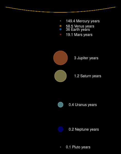
  p <- ggplot(my_planet_age, aes(x = sqrt(au), y = 1, size = radius, fill = planet, colour = planet)) +
    geom_point(alpha = 0.5, shape = 21, stroke = 1) +
    geom_text(aes(label = label, y = label_position), size = 5, hjust = 0, colour = "white") +
    geom_curve(aes(x = 0, y = 0, xend = 0, yend = 2), size = 0.3, curvature = 0.1,
               colour = "darkgoldenrod2") +
    scale_radius(range = c(0.5, 25)) +
    scale_x_reverse() +
    scale_colour_manual(values = planet_colours) +
    scale_fill_manual(values = planet_colours) +
    coord_flip() +
    theme_void() +
    theme(legend.position = "none",
          plot.background = element_rect(fill = "black"))
  
  return(p)
  
}

The my_planet_age_plot() again has your birthday and planet_data as its arguments, and firstly will call calc_my_planet_age() to produce the tibble of your planetary ages. Next we’ll define a colour scale (planet_colours) so that the colours of the planets are roughly equivalent to their colour⁶.

Now let’s build our plot p using {ggplot2}.

Using the my_planet_data object let’s first of all set the x-coordinate as the square root of the au variable, au is each planet’s distance from the Sun in Astronomical Units (where 1 AU is the distance from the Sun to Earth), we’ll use the square root to make the chart a little more practical. We’ll set all planets to have a y-coordinate of 1 so they’re all in a line (even though not-a-planet Pluto is on a very different plane to the main planets). Let’s then set the size of our planets as equal to their radius, and then the fill and colour to vary by planet name.

Having set our main options let’s now add the planets by using geom_point(), we’ll set all planets to have 50% transparency (alpha = 0.5) and to use the filled circle with an outline shape (shape = 21) so that the transparency applies to the fill but not the stroke, and we’ll set the stroke to have a weight of 1. And there we’ve plotted our planets (plus Pluto). We’ll add labels using geom_text(), setting the label to the label variable and y for these to the label_position varable we calculated with a position for each planet. We’ll also set the relative size of the text to 5, left-align the labels (hjust = 0) and make the text white in colour so that we can see it against the black background we’ll set. Finally, let’s use geom_curve() to add an outline trace for the sun.

That takes care of plotting our elements, next let’s style our plot. We can use scale_radius() to indicate that the size variable is actually for scaling the radii of our points rather than the area (which is the default), we can also set the range of point sizes that we want to scale our radii, in this case we’ve ranging from 0.5 to 25 so that the smallest planets are more visible in our plot. We’ll reverse the x-axis using scale_x_reverse() as we’re using coord_flip() to rotate the plot, this will ensure that the sun is at the top of the plot rather than the bottom. Next we’ll apply our custom planet colouring using scale_colour_manual() and scale_fill_manual(). Finally let’s remove all of ggplot’s base styling using theme_void(), and then strip the legend and set the plot_background to black using some custom theme() arguments.

And done, we’ve got a lovely planetary plot, which we return as an object to the user.

The sensor array (getting your next interplanetary birthday)

Our final helper is a function to extract the details of your next interplanetary birthday.

next_planet_birthday <- function(birthday, planet_data, what) {
  
  my_planet_age <- calc_my_planet_age(birthday, planet_data)
  
  next_birthday <- my_planet_age %>%
    filter(next_birthday_in == min(next_birthday_in))
  
  if (what == "where") {
    next_birthday_out <- next_birthday$planet
  } else if (what == "when") {
    next_birthday_out <- format(Sys.Date() + lubridate::days(next_birthday$next_birthday_in),
                                format = "%a %d %b %Y")
  } else if (what == "age") {
    next_birthday_out <- trunc(next_birthday$planetary_age) + 1
  }
  
  return(next_birthday_out)
  
}

As with our plotting function, next_planet_birthday() takes your birthday and planet_data as arguments and puts these in a call to calc_my_planet_age(). However, it also has a third argument: what, which will determine what information is extracted. First though, we’ll filter the data to the next planetary birthday by filtering the tibble to the smallest value of next_birthday_in (the number of Earth days until your next interplanetary birthday). Now we’ll look at the what argument and create output.

When what == "where" we want to know the planet your next birthday is on, this is a very simple extract of the value of the planet variable in our dataset.

When what == "when" we want to know when (on Earth) this birthday is we can do this by adding the number of days (next_birthday_in) to the current date (Sys.Date()). We can use the lubridate::days() function to ensure we’re taking account of leap days properly. Finally we wrap this around a call to format() so that we can format our date in a human readable format. This is specified by the format argument, here %a is the short form of the weekday (e.g. “Mon”), %d is the day (e.g. “01”), %b is the short form of the month (e.g. “Aug”) and %Y is the four-digit year (e.g. “2020”).

When what == "age" we want to know your age on your next interplanetary birthday, as with our calculation for finding the date we calculate this by rounding down your current interplanetary age and adding one.

The helm (setting up your UI)

Now that our helper functions have been written let’s create our ui object. The {shiny} package has a lot of helpful functions for creating layouts so that you don’t have to know any HTML or CSS (though it can help), it also has multiple types of page that you can create.

ui <- navbarPage("Interplanetary Birthday Express", tabPanel(
    emo::ji("alien"),
    fixedRow(column(
      12,
      fixedRow(column(
        4,
        fixedRow(column(
          12,
          HTML("Hello Human! I cake in peace!<br /><br />",
               "The planets in your solar system orbit the sun at different ",
               "rates, use this tool to find out how old you are on different ",
               "planets in your solar system!<br /><br />"),
          dateInput("birthday", "When is your birthday?", "2000-01-01"),
          HTML("Your next interplanetary birthday will be:<h2>"),
          textOutput("next_birthday_when", inline = TRUE),
          HTML("</h2> When you will be <strong>"),
          textOutput("next_birthday_age", inline = TRUE),
          HTML("</strong> years old on <strong>"),
          textOutput("next_birthday_where", inline = TRUE),
          HTML("</strong>")))),
        column(
          8,plotOutput("planet_plot", height = "600px"))))),
    fixedRow(column(
      12,
      HTML("<br />This tool represents the time since you were born ",
           "as years on each planet of the solar system, plus Pluto ",
           "(which isn't a planet but some of you like to think it is). ",
           "It does this by first converting the time since your birthday ",
           "into hours, this figure is then divided by the orbital period ",
           "of each planet in hours and rounded to one decimal place<br />",
           "<br />The sizes of the planets and their relative distance ",
           "from the sun are based on ",
           "<a href=\"https://nssdc.gsfc.nasa.gov/planetary/factsheet/index.html\">",
           "data from NASA</a>, but have been scaled to render in the plot.")))),
    fluid = FALSE)

In this example I’ve decided to use the navbarPage() format with rows and columns to create a grid for the content. I won’t go into detail of this set up, the main things to note are the dateInput(), textOutput() and plotOutput() which is where all the “app” work happens, the rest are blocks of HTML used to provide the rest of the user interface.

dateInput("birthday", "When is your birthday?", "2000-01-01")

The dateInput() function creates a date selector, we give it an id (“birthday”), a label (“When is your birthday?") and a default (“2020-01-01”, not my birthday) for it to use when the app first loads.

The textOutput() and plotOutput() functions are very simple calls for accessing the outputs from the Shiny app in their relevant form (textOutput() for text and plotOutput() for simple raster image plots), which you refer to by their relevant id. For plotOutput() I also specify a height to ensure the image is a specific height.

The warp core (the server function)

Now that we’ve made all our helper functions and designed our ui all that’s left to do is get the app moving, which we do via our server code. As I’ve abstracted all the calculation work to functions the code is very simple.

server <- function(input, output) {

  output$planet_plot <- renderPlot(
        my_planet_age_plot(input$birthday, planet_data)
    )
  
  output$next_birthday_where <- renderText(
    next_planet_birthday(input$birthday, planet_data, "where")
  )
  
  output$next_birthday_when <- renderText(
    next_planet_birthday(input$birthday, planet_data, "when")
  )
  
  output$next_birthday_age <- renderText(
    next_planet_birthday(input$birthday, planet_data, "age")
  )
}

A Shiny server is a function that has input and output arguments, and in essence your code is creating entities within the output object. First we create the planet_plot entity within output as a call to the my_planet_age_plot() function, using the birthday entity within input. We wrap this inside renderPlot() so that Shiny knows that when any of the values in input are updated that it should redraw the plot. We then also create output entities called next_birthday_where, next_birthday_when and next_birthday_age which will call the next_planet_birthday() function and get the relevant text. As with our plot these are wrapped in a call to renderText() so that Shiny knows to update the text. Our calls in the ui to plotOutput() and textOutput() use the names of these entities as the “id” that they use to display the relevant output.

Finally we run the application with a single line of code:

shinyApp(ui = ui, server = server)

Deploying the Shiny App to shinyapps.io

The app we’ve built can run on our machine, but if we want others to see/use it then we need to host it somewhere. For personal projects I’m using the free version of shinyapps.io because (a) it’s free, (b) it’s easily supported from within RStudio.

When you first use shinyapps.io you’ll be given a snippet of R code to set the credentials on your machine to access the shinyapps.io server.

rsconnect::setAccountInfo(name="<ACCOUNT>", token="<TOKEN>", secret="<SECRET>")

You then deploy your Shiny app using another single line of code:

rsconnect::deployApp()

Whenever you modify or update your app you just need to re-run the deployApp() command and your shinyapp.io app will be updated.

If you’re version controlling your app with GitHub make sure to add rsconnect/ and .secrets to your .gitignore file to ensure these are not accidentally sent to the cloud, especially important if it’s a public repo.

Finally, one strange thing I discovered was that while it was fine on my machine once deployed to the web my Shiny app had issues reading the .CSV file of planet_data, so I saved it as a .RDS file and then it worked.

So there we have it, the Interplanetary Cake Union now has a handy app to help remind you to order more cake from their Interplanetary Birthday Express Service⁷.