My last post explored using the {tidymodels} package with data about the Eurovision Song Contest1. One of the best things to do when exploring a dataset is to visualise it, so let’s also use this dataset to learn about the {gganimate} package that provides ways to create animated charts.
We’ll reuse the eurovision_scores dataset produced from the code in my last post. First let’s take a look at UK performance over time, we also need to filter out data from 1991 where Sweden and France both gained 146 points (but due to the complex rules in place at the time Sweden won, however under the current rules France would have won).
gb_scores <- eurovision_scores %>%
  filter(country == "GBR") %>%
  filter(!(year == 1991 & winning_country == "FRA")) %>%
  select(year, UK = score, Winner = winning_score) %>%
  pivot_longer(cols = -year, names_to = "country", values_to = "score")
First let’s create a generic plot of the scores over time, which we can use as the basis for our animation.
p_line <- ggplot(gb_scores, aes(x = year, y = score, colour = country)) +
  geom_line() +
  geom_point() +
  labs(title = "UK and winning country's Eurovision scores 1975-2019",
       x = "Year",
       y = "Score") +
  scale_colour_manual(values = c("Winner" = "goldenrod2", "UK" = "dodgerblue3")) +
  mattR::theme_lpsdgeog() +
  theme(
    plot.title = element_text(lineheight = 1.1),
    legend.title = element_blank(),
    legend.position = "bottom"
  )
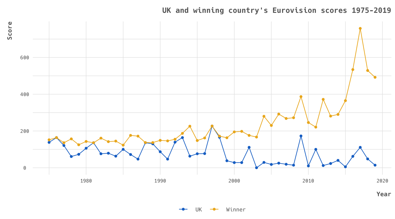
UK and winning country’s scores in the Eurovision final 1975-2019
{gganimate} provides a similar syntax to {ggplot2} that allows us to easily animate our charts. We can use the transition_reveal function to progressively build an animation where the line element persists across the animations. All we need to do is provide a single argument to this function that is the the name of the column in the data that we wish to use as the feature that animates the data, the year. Through my tests I’ve found it common sense to specify the pixel size of the animation you want before you save it, which you do by setting gganimate.dev_args in a call to options().
library(gganimate)

anim_line <- p_line +
  transition_reveal(year)

options(gganimate.dev_args = list(width = 900, height = 900*9/16))
anim_save("eurovision_uk_winner.gif", anim_line, fps = 5)
UK and winning country’s scores in the Eurovision final 1975-2019 (animated)
Animations can also be applied to maps, allowing us to visualise Eurovision scores over time. First let’s get country outlines via the {rnaturalearth} package. We’ll also subset these to clip out everything west of Iceland and everything east of Australia. Then we can merge in our eurovision_scores data. As we saw from the previous chart in recent years the winner’s score has massively increased, so let’s again calculate the relative score for each country.
world_countries <- rnaturalearth::ne_countries(returnclass = "sf")

world_cropped <- sf::st_crop(world_countries, xmin = -30, xmax = 155, ymin = -90, ymax = 90)

eurovision_countries <- world_cropped %>%
  filter(iso_a3 %in% unique(eurovision_scores$country)) %>%
  left_join(eurovision_scores, by = c("iso_a3" = "country")) %>%
  mutate(relative_score = score/winning_score)
Again, let’s construct a basic plot, this time with 2019 data, to ensure we’re laying out our map correctly.
p_map1 <- ggplot(eurovision_countries %>% filter(year == 2019)) +
  geom_sf(aes(fill = relative_score), size = 0.1, colour = "grey90") +
  scale_fill_gradient(low = "dodgerblue3", high = "goldenrod2",
                      guide = guide_none()) +
  labs(
    title = "Relative scores in the Eurovision Finals: 2019",
    subtitle = "Relative score = country score / winning score"
  ) +
  mattR::theme_lpsdgeog(subtitle = TRUE) +
  theme(
    axis.text = element_blank()
  )
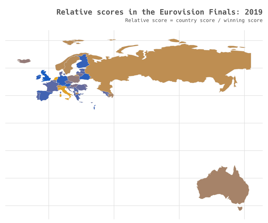
Map of Eurovision 2019 final scores
Animating this is again relatively simple, however you need to make sure you have installed the {transformr} package which is needed for animating ggplot2::geom_sf() objects. This time we’ll use the transition_state() animation function, again it requires a single argument (in our case year). However, let’s revise our plot object first, removing the filtering of the data to just the 2019 scores, and adding in a {glue} style call to transition information in the title text so that we can reference the year in the title of the chart/
p_map2 <- ggplot(eurovision_countries) +
  geom_sf(aes(fill = relative_score), size = 0.1, colour = "grey90") +
  scale_fill_gradient(low = "dodgerblue3", high = "goldenrod2",
                      guide = guide_none()) +
  labs(
    title = "Relative scores in the Eurovision Finals: {closest_state}",
    subtitle = "Relative score = country score / winning score"
  ) +
  mattR::theme_lpsdgeog(subtitle = TRUE) +
  theme(
    axis.text = element_blank()
  )

anim_map <- p_map2 +
  transition_states(year) +
  theme(
    plot.title = element_text(size = 16),
    axis.title = element_text(size = 14),
    axis.text = element_text(size = 12),
    legend.text = element_text(size = 12)
  )

options(gganimate.dev_args = list(width = 750, height = 610))
anim_save("eurovision_timeseries", anim_map, fps = 5)

Animated map of scores in the Eurovision finals 1975-2019
I’m pleasantly surprised by just how easy it is to get started with {gganimate}. If I was going to improve this further I’d crop Russia east of the Urals and perhaps relocate Australia a little closer so that we can zoom in on Europe and see the variation in European countries a bit better, but that’s for another day (should I ever get round to it).