
Last Saturday, Saturday 16th May 2020 was scheduled to be the 65th Eurovision Song Contest, but due to the ongoing COVID19 pandemic the contest was cancelled. Eurovision is very special to me, and I’ve been lucky to attend a couple of the finals and semi-finals – and, if you were watching the second semi-final of the 2015 contest you may have even seen me on TV! I’ve recently watched some of Julia Silge’s TidyTuesday webcasts using the {tidymodels} framework, and so instead of watching the EBU’s tribute show and getting rather sad about the contest not happening and Daði Freyr not winning and giving me an even better excuse to go back to Iceland1 I decided to play with {tidymodels} and the Datagraver’s Eurovision points dataset on Kaggle.
Exploring the dataset
Firstly, let’s familiarise ourselves with the dataset. Using the {readxl} package we can inspect the the Excel document to understand that their are three three sheets (data, remarks and sources), the second and third sheet are just notes and metadata. The first sheet is a dataset that shows for the years 1975 to 2019 the points given by each country to each other country, so let’s read that in and inspect it.
readxl::excel_sheets("eurovision_song_contest_1975_2019.xlsx")

eurovision_raw <- readxl::read_excel(
  path = "eurovision_song_contest_1975_2019.xlsx",
  sheet = "Data"
)
The dataset has eight columns:
Year: the year of the contest(semi-) final: flag for whether it is the semi-final or final showEdition: a combination of Year and showJury or Televoting: the source of the votesFrom country: the country giving the pointsTo country: the country receiving the pointsPoints: the number of points awardedDuplicate: a marker that shows when the from and to country are the same
> eurovision_raw

| Year|(semi-) final |Edition |Jury or Televoting |From country         |To country | Points|Duplicate |
|----:|:-------------|:-------|:------------------|:--------------------|:----------|------:|:---------|
| 1980|f             |1980f   |J                  |Italy                |Spain      |      6|NA        |
| 1986|f             |1986f   |J                  |Cyprus               |Austria    |      0|NA        |
| 2008|f             |2008f   |J                  |Serbia               |Greece     |      8|NA        |
| 2009|sf1           |2009sf1 |J                  |United Kingdom       |Belarus    |      0|NA        |
| 2012|f             |2012f   |J                  |Cyprus               |Sweden     |     10|NA        |
| 2014|sf2           |2014sf2 |J                  |Romania              |Georgia    |      0|NA        |
This is a fairly tidy dataset to start with, but what’s the fun of leaving things as they are, it’d certainly be easier with tidy column names, at least. We can get rid of those duplicate rows, there’s also a typo in some of the rows where The Netherlands is missing the ’l’. Due to increasing participation from Eastern European countries, a semi-final was introduced in 2004 but this was quickly replaced by two semi-finals that select all but six of the finalists (the host country and the five largest funders of the European Broadcasting Union: France, Germany, Italy, Spain and the United Kingdom). This is recorded in the second and third columns, but let’s add a generic flag for whether it’s a final or semi-final.
eurovision_proc <- eurovision_raw %>%
  janitor::clean_names() %>%
  filter(is.na(duplicate)) %>%
  select(-duplicate) %>%
  rename(show = semi_final,
         vote_type = jury_or_televoting) %>%
  mutate_at(vars(from_country), ~str_replace(., "The Netherands", "The Netherlands")) %>%
  mutate(
    show_type = as_factor(if_else(show == "f", "final", "semi-final")),
    show = fct_recode(show,
                      "final" = "f",
                      "single-semi" = "sf",
                      "semi-one" = "sf1",
                      "semi-two" = "sf2"),
    vote_type = fct_recode(vote_type,
                           "jury" = "J",
                           "televote" = "T"))
> eurovision_proc

| year|show     |edition |vote_type |from_country |to_country       | points|show_type  |
|----:|:--------|:-------|:---------|:------------|:----------------|------:|:----------|
| 2009|final    |2009f   |jury      |Slovakia     |Greece           |      0|final      |
| 1980|final    |1980f   |jury      |Greece       |Portugal         |      5|final      |
| 2019|final    |2019f   |jury      |Estonia      |Italy            |      0|final      |
| 2016|semi-two |2016sf2 |televote  |Belgium      |F.Y.R. Macedonia |      0|semi-final |
| 2017|final    |2017f   |jury      |Denmark      |Belgium          |      2|final      |
| 2016|semi-one |2016sf1 |televote  |Finland      |Russia           |      8|semi-final |
I’m also a big fan of country-codes rather than country names, especially in large data, so we can use my good friend the {countrycode} package. However, as our data goes back to 1975 we’ve actually got two sets of country names that don’t appear in the current set of country codes: Yugoslavia and Serbia & Montenegro. So let’s build a custom function to make sure these get their historic country code.
eurovision_country_code <- function(x) {

  code <- case_when(
    x == "Serbia & Montenegro" ~ "SCG",
    x == "Yugoslavia" ~ "YUG",
    TRUE ~ countrycode::countrycode(x, "country.name", "iso3c")
  )

  return(code)

}
We can now apply this function to our data to convert the country names in the fifth and sixth columns into country codes.
eurovision_dt <- eurovision_proc %>%
  mutate_at(vars(from_country, to_country), eurovision_country_code)
> eurovision_dt

| year|show        |edition |vote_type |from_country |to_country | points|show_type  |
|----:|:-----------|:-------|:---------|:------------|:----------|------:|:----------|
| 1994|final       |1994f   |jury      |GRC          |RUS        |      4|final      |
| 2018|final       |2018f   |televote  |SVN          |ALB        |      1|final      |
| 1977|final       |1977f   |jury      |FRA          |CHE        |      0|final      |
| 2006|single-semi |2006sf  |jury      |ALB          |BGR        |      8|semi-final |
| 2003|final       |2003f   |jury      |TUR          |BEL        |      7|final      |
| 2012|semi-one    |2012sf1 |jury      |ISL          |CYP        |     12|semi-final |
Points are all well and good, and points do mean prizes, but only once we totalise them into scores, we also want to get information about winners. We could produce these as separate tables, or we could write some functions and apply them to the data using {purrr}. Let’s define a function calc_scores() to total up the points received by a country to get their overall score, this function groups a tibble by to_country and then create a new score column that is a sum of the points column, this will then return a 2-column dataset of to_country and score. The get_winner() function takes the scores dataset returned by calc_scores() and filters it for the row with the highest score, as we’ll ultimately merge this back into our data in a latter step the columns are renamed winning_country and winning_score.
calc_scores <- function(data) {

  scores <- data %>%
    group_by(to_country) %>%
    summarise(score = sum(points)) %>%
    ungroup()

  return(scores)

}

get_winner <- function(data) {

  winner <- data %>%
    filter(score == max(score)) %>%
    rename(winning_country = to_country, winning_score = score)

  return(winner)

}
To use these functions we need to group our dataset by year and show, and create a nested data-frame with the type of vote, country information and points columns. We can then use purrr::map() the apply calc_scores() to the data, and get_winner() to the scores we have calculated. After un-nesting these new columns we can then do some additional processing, identifying if a country was the winner that year/show. We can also calculate how many wins (since 1975) a country has had using the cumulative sum (cumsum()) function, although we should net 1 from any scores because their first win shouldn’t count.
eurovision_scores <- eurovision_dt %>%
  group_by(year, show) %>%
  nest(data = c(vote_type, from_country, to_country, points)) %>%
  mutate(
    scores = map(data, calc_scores),
    winner = map(scores, get_winner)) %>%
  select(-data) %>%
  unnest(winner) %>%
  unnest(scores) %>%
  mutate(
    show_winner = winning_country == to_country,
    outcome = case_when(
      show_winner & show_type == "final" ~ "win-final",
      show_winner & show_type == "semi-final" ~ "win-semi",
      TRUE ~ "no-win"
    )) %>%
  rename(country = to_country) %>%
  group_by(country) %>%
  mutate(prev_wins = cumsum(overall_winner)) %>%
  ungroup() %>%
  mutate(prev_wins = if_else(prev_wins > 0, prev_wins - 1, 0))
> eurovision_scores

| year|show     |edition |show_type  |country | score|winning_country | winning_score|show_winner |outcome   |overall_winner | prev_wins|
|----:|:--------|:-------|:----------|:-------|-----:|:---------------|-------------:|:-----------|:---------|:--------------|---------:|
| 1986|final    |1986f   |final      |IRL     |    96|BEL             |           176|FALSE       |no-win    |FALSE          |         0|
| 2019|semi-one |2019sf1 |semi-final |SVN     |   165|AUS             |           260|FALSE       |no-win    |FALSE          |         0|
| 1991|final    |1991f   |final      |FRA     |   146|SWE             |           146|FALSE       |no-win    |FALSE          |         1|
| 1979|final    |1979f   |final      |DNK     |    76|ISR             |           125|FALSE       |no-win    |FALSE          |         0|
| 2009|final    |2009f   |final      |NOR     |   387|NOR             |           387|TRUE        |win-final |TRUE           |         2|
| 2017|semi-one |2017sf1 |semi-final |CZE     |    83|PRT             |           370|FALSE       |no-win    |FALSE          |         0|
Preparing to model the data
At present our dataset just has the overall score for a country and other meta-data. The only potential ‘predictor’ that we have in the data is prev_wins, and that might be interesting. But let’s think creating a model, the data goes all the way back to 1975 but semi-finals started getting used in 2004 so let’s actually just create a model based on the data relating to the finals. Something that is oft-cited in Eurovision is that countries always vote for their neighbours, so perhaps it might be interesting to model data related to neighbours. At the moment we don’t have any information that tells us who are neighbours, I’m not aware of an R package that has this, so I found this wikipedia page that provides a table of countries by land borders, including a column with the countries that have borders. We can import this using {rvest} and it’s html_table() function to convert the table into an R data structure.
wiki_url <- "https://en.wikipedia.org/wiki/List_of_countries_and_territories_by_land_borders"

wiki_page <- xml2::read_html(wiki_url)
wiki_tbl <- wiki_page %>%
  rvest::html_nodes("table") %>%
  pluck(1) %>%
  rvest::html_table(fill = TRUE)
This data isn’t particularly clean, while the final column of this table contains a list of neighbouring countries, this is all as a single row. So let’s write a function to extract these as separate rows, which we can again apply to the tibble via purrr::map(). While we’re at we can also clean up the column titles, clean the country names (dropping footnote references, dealing with the multiple rows for the UK and France) and convert the country names to country codes.
get_neighbours <- function(data) {

  data <- data %>%
    str_remove_all("Includes:|\\[\\d+\\]") %>%
    str_split("\\n|:|\\)", simplify = TRUE) %>%
    str_trim()

  extract <- data %>%
    map_lgl(~str_detect(., "^\\d|^$", negate = TRUE))

  neighbour_codes <- data[extract] %>%
    countrycode::countrycode("country.name", "iso3c") %>%
    tibble::enframe(name = NULL) %>%
    set_names("neighbour")

  return(neighbour_codes)

}

neighbours <- wiki_tbl[-1,] %>%
  set_names(c("country", "total_length_km", "total_length_mi", "num_borders", "num_neighbours", "neighbours")) %>%
  select(country, neighbours) %>%
  mutate(
    country = str_remove_all(country, "\\n.*$|\\[\\d+\\]| \\(People's Republic of China\\)"),
    country = case_when(
      str_detect(country, "France.*excl") ~ "France",
      str_detect(country, "France.*excl") ~ "France+DOM",
      str_detect(country, "United.*plus") ~ "UK+BOT+CD",
      TRUE ~ country),
    country_code = countrycode::countrycode(country, "country.name", "iso3c"),
    neighbours = map(neighbours, get_neighbours)) %>%
  drop_na(country_code) %>%
  select(country = country_code, neighbours) %>%
  unnest(neighbours) %>%
  drop_na()
This results in a two-column table that matches a country with it neighbour.
> neighbours %>% filter(country %in% c("GRC", "NOR"))

|country |neighbour |
|:-------|:---------|
|GRC     |ALB       |
|GRC     |BGR       |
|GRC     |TUR       |
|GRC     |MKD       |
|NOR     |FIN       |
|NOR     |SWE       |
|NOR     |RUS       |
In reviewing the output table there’s a bit of complexity, notably the case of European countries’ overseas territories and whether these territories’ borders with other European countries count as the countries being neighbours even though their European territories don’t share a border, such as the Franco-Dutch land-border in the Caribbean. For the sake of simplicity, I went with yes. There’s also asymmetry in the table, the UK’s row lists Ireland as it’s only land neighbour, yet the rows for Cyprus and Spain list the UK as a neighbour (because of the UK sovereign base areas in Cyprus and Gibraltar’s border with Spain).
> neighbours %>% filter(country == "GBR" | neighbour == "GBR")

|country |neighbour |
|:-------|:---------|
|CYP     |GBR       |
|IRL     |GBR       |
|ESP     |GBR       |
|GBR     |IRL       |
To solve this problem, let’s flip the table, append it to our original table and remove duplicates.
neighbours2 <- neighbours %>%
  rename(country = neighbour, neighbour = country) %>%
  select(country, neighbour) %>%
  bind_rows(neighbours)

neighbour_list <- neighbours2 %>%
  select(country, neighbour) %>%
  distinct() %>%
  arrange(country, neighbour)
This now gives us four rows with GBR as a country and four as a neighbour.
> neighbour_list %>% filter(country == "GBR" | neighbour == "GBR")

|country |neighbour |
|:-------|:---------|
|CYP     |GBR       |
|ESP     |GBR       |
|GBR     |CYP       |
|GBR     |ESP       |
|GBR     |IRL       |
|IRL     |GBR       |
Now we’ve a list of neighbours we can do several things: calculate the number of neighbours a country has, the number of points a country received from it’s neighbours, and the points it gave to it’s neighbours. The first set of data can be easily calculated via a call to the dplyr::count() function which handily summarises the frequency of observations in a tibble.
num_neighbours <- neighbour_list %>%
  count(country) %>%
  rename(num_of_neighbours = n)
> num_neighbours

|country | num_of_neighbours|
|:-------|-----------------:|
|CYP     |                 1|
|CRI     |                 2|
|SWE     |                 3|
|UGA     |                 5|
|FRA     |                 8|
|IND     |                 9|
To calculate the points to/from neighbours we can write a function to use our table to compare whether two countries are neighbours and apply that to our original voting data.
check_neighbour <- function(from_country, to_country) {

  neighbours <- neighbour_list %>%
    filter(country == from_country) %>%
    pull(neighbour)

  check <- (to_country %in% neighbours)

  return(check)

}

points_from_neighbours <- eurovision_dt %>%
  mutate(neighbour = map2_lgl(from_country, to_country, check_neighbour)) %>%
  filter(neighbour) %>%
  group_by(year, show, to_country) %>%
  summarise(points_from_neighbours = sum(points)) %>%
  ungroup() %>%
  rename(country = to_country)

points_to_neighbours <- eurovision_dt %>%
  mutate(neighbour = map2_lgl(from_country, to_country, check_neighbour)) %>%
  filter(neighbour) %>%
  group_by(year, show, from_country) %>%
  summarise(points_to_neighbours = sum(points)) %>%
  ungroup() %>%
  rename(country = from_country)
> points_from_neighbours

| year|show     |country | points_from_neighbours|
|----:|:--------|:-------|----------------------:|
| 2009|semi-one |BEL     |                      0|
| 2014|final    |FRA     |                      0|
| 2013|semi-one |SRB     |                     20|
| 2014|semi-one |AZE     |                     10|
| 1979|final    |AUT     |                      4|
| 2001|final    |POL     |                      5|
Let’s calculate the total number of points given by a country in a given show.
points_given <- eurovision_dt %>%
  group_by(year, show, from_country) %>%
  summarise(points_given = sum(points)) %>%
  ungroup() %>%
  rename(country = from_country)
> points_given

| year|show  |country | points_given|
|----:|:-----|:-------|------------:|
| 1995|final |DNK     |           58|
| 2004|final |ROU     |           58|
| 2006|final |CYP     |           58|
| 2014|final |GRC     |           58|
| 2016|final |ITA     |          116|
| 2019|final |SMR     |          114|
Planning our model
Now that we’ve calculated these additional metrics, let’s now think about modelling and assembling a final dataset. To use the full range of data let’s think about modelling the outcomes of the finals, since that data goes back to 1975. We can subset our eurovision_scores dataset to just the finals, we can merge the number of neighbours and the points from/to neighbours data. This would allow us to construct a basic model, but let’s calculate some further metrics. Firstly, since the number of participating countries has grown over time, so too has the winning score, let’s sort this out by calculating a relative score where a country’s score is a proportion of the winning score.
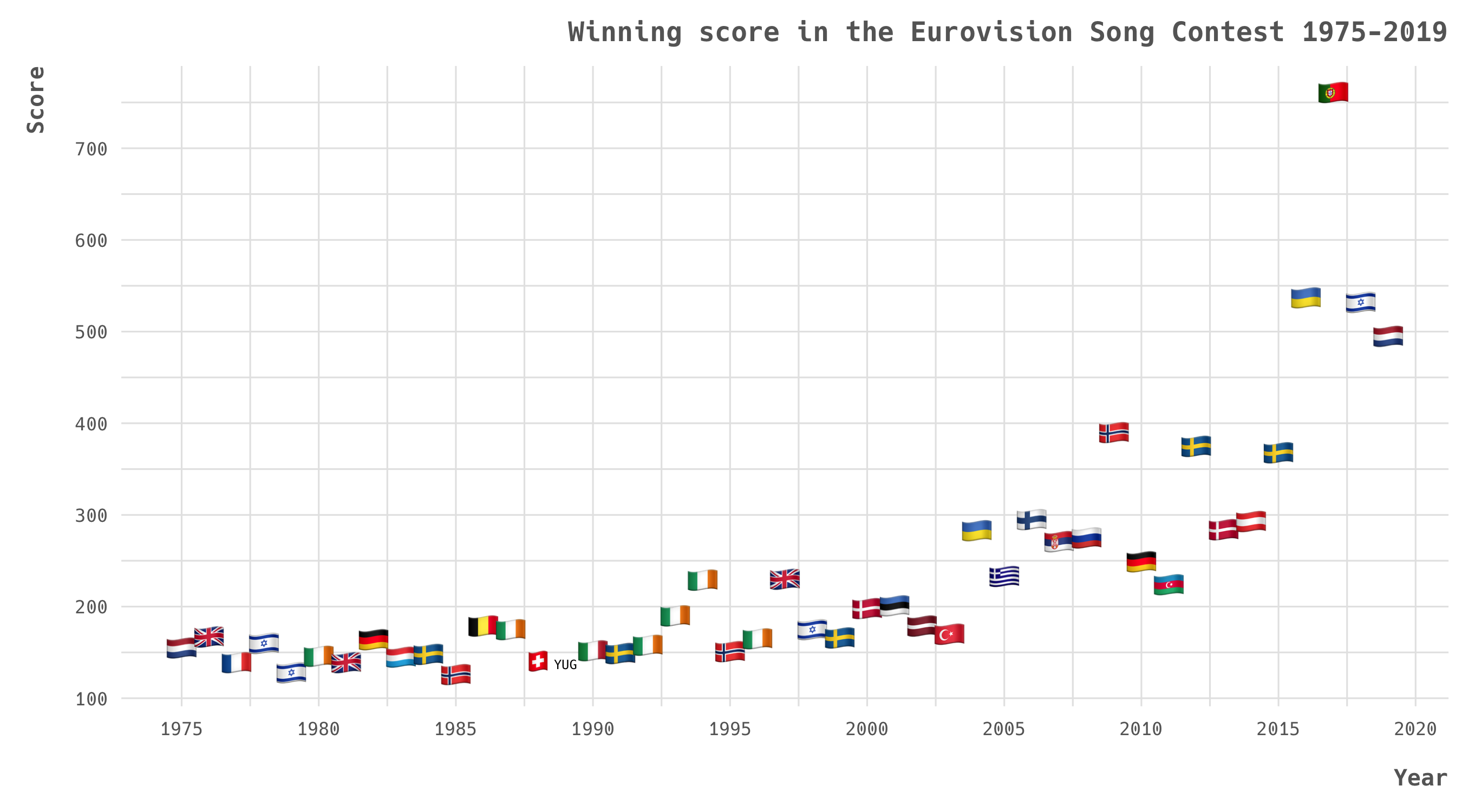
Eurovision winning scores 1975-2019
We can also convert our points to/from neighbours into relative scores. Let’s call the proportion of a country’s points from its neighbours its friendly score (i.e. the more friendly you are the more of your points will come from your neighbours). Let’s calculate the proportion of the points given by a country to its neighbours, and call this neighbourly (i.e. as a good neighbour you will give more of your points to your neighbours). For each of these measures let’s calculate a ‘dispersion’ factor, that is your friendly/neighbourly scores divided by the number of neighbours. Finally let’s calculate a kinship measure which combines both the points given and received, which we will calculate as the square root of the product of the points to and from neighbours and then divided by the number of neighbours.
eurovision_final_scores <- eurovision_scores %>%
  filter(show_type == "final") %>%
  left_join(num_neighbours) %>%
  left_join(semi_results) %>%
  left_join(points_from_neighbours) %>%
  left_join(points_to_neighbours) %>%
  left_join(points_given) %>%
  select(year, country, score, winning_score, show_winner,
         semi_winner = semi_outcome, prev_wins, num_of_neighbours,
         points_from_neighbours, points_to_neighbours, points_given) %>%
  mutate(
    show_winner = as_factor(if_else(show_winner, "winner", "participant")),
    semi_winner = case_when(
      year >= 2004 & is.na(semi_winner) ~ FALSE,
      TRUE ~ semi_winner),
    relative_score = score/winning_score,
    friendly = points_from_neighbours/score,
    friendly_dispersion = friendly/num_of_neighbours,
    neighbourly = points_to_neighbours/points_given,
    neighbourly_dispersion = neighbourly/num_of_neighbours,
    kinship = sqrt(points_from_neighbours * points_to_neighbours) /
      num_of_neighbours
  ) %>%
  mutate_if(is.numeric, replace_na, 0) %>%
  mutate_if(is.numeric, ~if_else(is.infinite(.), 0, .))
Let’s now define a hypothetical model that a country’s relative score and/or its likelihood of winning is proportionate to its friendliness, neighbourliness, the dispersion of these two metrics, its kinship and its number of previous wins since 1975.
outcome [relative_score | show_winner] ~ friendly + friendly_dispersion + neighbourly + neighbourly_dispersion + kinship + prev_wins
Running the regression models
Now let’s finally get to our experiments with the {tidymodels} framework. Just as with the {tidyverse} we can easily load the relevant packages with a simple call: library(tidymodels}. The tidymodels framework is designed at its core to enable model training and testing, while we won’t do any complex model training it can still be useful to apply these principles to general modelling. So let’s split our dataset into training and testing data, by default we’ll use 75% of our data for training and 25% for testing. Before splitting our data let’s set the random seed so that this analysis is reproducible, and let’s use the expected date of the 2020 Eurovision final as our seed value. The {rsample} package can neatly split our datasets and create training and testing data, in splitting the data we can also define a strata that allows us to ensure the training and testing data have a similar proportion of Eurovision show winners.
set.seed(20200516)

eurovision_split <- rsample::initial_split(eurovision_final_scores, strata = show_winner)

eurovision_train <- rsample::training(eurovision_split)
eurovision_test <- rsample::testing(eurovision_split)
Having split our data we can now define our model, which we do using the recipe() function from the {recipes} package. This ensures we’ve defined our model in the right format, let’s define two recipes, one for a linear model where we’re using the relative_score as our outcome variable and one for a logistic model where show_winner is the outcome variable.
relscore_rec <- recipes::recipe(relative_score ~ friendly + friendly_dispersion +
                                neighbourly + neighbourly_dispersion + kinship +
                                prev_wins, data = eurovision_train)

winner_rec <- recipes::recipe(show_winner ~ friendly + friendly_dispersion +
                              neighbourly + neighbourly_dispersion + kinship +
                              prev_wins, data = eurovision_train)
Now let’s define the modelling engines which we can do using functions from the {parsnip} package, which provides a common API for handling common modelling approaches. In these cases we’re using the built-in modelling ’engines’ of stats::lm() for linear regression and stats::glm() for logisitic regresison, but {parsnip} provides a common interface for using many other modelling algorithms without requiring you to learn the different syntax associated with each algorithm’s relevant package.
lm_mod <- linear_reg() %>%
  set_engine("lm")

lr_mod <- logistic_reg() %>%
  set_engine("glm")
Now that we’ve defined our models’ recipes and set the modelling engines, we can create a workflow for each model and then fit that workflow to model the data.
relscore_wflow <- workflow() %>%
  add_model(lm_mod) %>%
  add_recipe(relscore_rec)

relscore_fit <- relscore_wflow %>%
  fit(data = eurovision_train)

winner_rec_wflow <- workflow() %>%
  add_model(lr_mod) %>%
  add_recipe(winner_rec)

winner_rec_fit <- winner_rec_wflow %>%
  fit(data = eurovision_train)
We can review the coefficients of these models by ‘pulling’ the results from the fit and then using broom::tidy() to present the results as a tibble. We can see from this that a country’s relative_score does not have a statistically significant relationship with the number of previous wins, but that neighbourliness is positively correlated with your relative score, while the proportion of points received from your neighbours is inversely related to your relative score.
> relscore_fit %>% workflows:: pull_workflow_fit() %>%
  broom::tidy()

|term                   |   estimate| std.error|  statistic|   p.value|
|:----------------------|----------:|---------:|----------:|---------:|
|(Intercept)            |     0.3451|    0.0145|    23.7296|    0.0000|
|friendly               |    -0.3827|    0.0723|    -5.2917|    0.0000|
|friendly_dispersion    |    -0.3497|    0.1627|    -2.1490|    0.0319|
|neighbourly            |     0.2622|    0.0970|     2.7007|    0.0070|
|neighbourly_dispersion |    -2.3254|    0.3217|    -7.2264|    0.0000|
|kinship                |     0.0665|    0.0050|    13.1089|    0.0000|
|prev_wins              |    -0.0026|    0.0104|    -0.2503|    0.8024|
However, the logistic model shows different results: your number of previous wins has a slight increase in the likelihood of winning, while a country distributing points to its neighbours (our neighbourly metric) has no statistically significant effect on your chances of winning. Similarly, the proportion of points recieved from neighbours has no significant effect on your chances of winning, but the dispersion of this (i.e. getting points from a lot of your neighbours) and your kinship levels (giving and receiving points from neighbours) do have statistically significant effects on your chances of winning Eurovision.
>winner_rec_fit %>% workflows::pull_workflow_fit() %>%
  broom:: tidy()

|term                   |    estimate|  std.error|  statistic|   p.value|
|:----------------------|-----------:|----------:|----------:|---------:|
|(Intercept)            |  -3.4583145|  0.3591681| -9.6286799| 0.0000000|
|friendly               |   0.6548786|  3.2649293|  0.2005797| 0.8410272|
|friendly_dispersion    | -34.9105876| 16.5517699| -2.1091755| 0.0349294|
|neighbourly            |   1.6269553|  2.4676206|  0.6593215| 0.5096894|
|neighbourly_dispersion | -16.9454316| 10.0068589| -1.6933817| 0.0903828|
|kinship                |   0.5864228|  0.1085535|  5.4021557| 0.0000001|
|prev_wins              |   0.4067809|  0.1836427|  2.2150670| 0.0267555|
Having now fit our models, let’s now test whether they are actually useful and robust models that we can draw conclusions from, we can do this using the {yardstick} package. First let’s use our fitted models to predict outcomes in our test data.
relscore_test <- relscore_fit %>%
  predict(new_data = eurovision_test) %>%
  mutate(truth = eurovision_test$relative_score)

winner_test <- winner_rec_fit %>%
  predict(new_data = eurovision_test) %>%
  mutate(truth = eurovision_test$show_winner)
We can then use these predicted outcomes to test the efficacy of our models. For linear regression we can easily calculate the standard model fitting statistics of R-square and root mean standard error. These suggest that the model is providing some level of accuracy, in that it explains around 21% of the variation in relative scores, and has a relatively low level of standard error.
> relscore_test %>% rsq(truth = truth, estimate = .pred)
0.208

> relscore_test %>% rmse(truth = truth, estimate = .pred)
0.249
The accuracy and positive predictive value measures from the logistic regression are encouraging, suggesting that the model is accurate around 94% of the time.
> winner_test %>% accuracy(truth = truth, estimate = .pred_class)
0.943

> winner_test %>% ppv(truth = truth, estimate = .pred_class)
0.950
However, when we investigate further we can see that this is driven by correctly predicting that countries did not win Eurovision, and the model failed to predict any actual winners.
> winner_rec_test %>% count(.pred_class, truth)

|.pred_class |truth       |   n|
|:-----------|:-----------|---:|
|participant |participant | 248|
|participant |winner      |  13|
|winner      |participant |   2|
Reviewing {tidymodels}
This example wasn’t about generating useful analysis of the Eurovision results (much as that is an interesting topic, and the subject of a couple of PhDs), but rather an experiment in using the {tidymodels} framework. In general, it feels like a useful framework that makes it easy to apply the same approach to modelling when using both linear and logistics regression models. While stats::lm() and stats::glm() have similar syntax, the tidymodels framework integrates neatly with the wider {tidyverse} family of packages. As I said at the outset, I’ve watched a couple of Julia Silge’s TidyTuesday webcasts which certainly demonstrate the power of the {tidymodels} framework, and the work to write this blog has demostrated that it’s relatively easy to pick up the basics of these packages.
-
I’d also be totally fine with The Mamas from Sweden’s Move winning.
I’m always impressed by Latvia’s tendency to submit heavy-beats-Euro-RnB entries, this year’s Still Breathing by Samanta Tina is very strong. Fellow Latvian Aminata’s 2015 entry Love Injected remains one of my most favourite ESC songs ever (though admittedly not very Eurovision) and experiencing it live was a truly transcendant moment, there were some great club versions that seem to have disappeared from the internets. Ukraine are always a very strong competitor, and this year they have provided a fabulous with Go_A’s electro-dance-folk bop [Solovey], and while it’s no Wild Dance or Shady Lady2, or as legendary a performance as that provided by Verka Serduckha it’s a good piece. However, in selecting The Roop’s On Fire, Lithuania’s national selection process has robbed us of one of the best Eurovision lyrics ever “don’t forget to water my plants when I’m gone”, plus strong neon looks. Australia always deserves an honourable mention, not just because they always put in strong entries but also because of their love and dedication to a contest that takes place on the other side of the planet that they are willing to get up at 5am on a Sunday morning to watch it; however this year’s entry by Montaigne is good, however it will be very difficult for an Aussie act to top Dami Im’s 2016 entry Sound of Silence which was robbed (and the UK’s best chance of hosting the contest in 20 years). ↩︎ -
There is a vicious rumour that back in 2008, when it was still costly to televote, I drunkenly spent £30 calling in to try and get the UK to give this douze points3. ↩︎
-
All rumors are based in truth, a truth that I will only admit when at a similar level of inebriation. I might also have been trying to impress a boy by demonstrating my commitment to Eurovision4. ↩︎
-
It worked. ↩︎