
No matter what job we do or who we work for all of us have been in meetings that we knew weren’t worth it. For those of us in the public sector there’s the added pressure knowing that we’re paid by the taxpayer. A couple of weeks ago a friend who works in another government department (for arguments sake the Department for Action) was lamenting that they and their team of six were asked by a someone in another government department (let’s say the Ministry of Meetings) to have a meeting with their team about a joint project they were working on. Come the time of the meeting my friend in DfA and her team all signed on to the virtual meeting, 10-15 minutes go by and none of the folk from MoM turn up. Not only is this wasted time, but time also means money, and in this case public money.
When complaining to me about the saga my friend mentioned the Meeting Cost Calculator that had been developed by some Canadian public servants, and mused that wouldn’t it be nice if we could have one in the UK so that they could send a bill our friends in MoM for the cost to DoD of their no-show. And so, I made an entirely unofficial HMG Meeting Cost Calculator to estimate the cost of meetings of civil servants in the UK1.
She works hard for the money: getting the data
The Cabinet Office publishes an annual statistical release, the Civil Service Statistics, which includes a range of information about the salaries/pay of civil servants2. The data is published as an Open Document Spreadsheet (ODS) file, which while an open format does not mean that the data contained in the document is necessarily machine readable. First thing’s first, download the file, which we can do programatically using the download.file() from R’s core {utils} package.
library(tidyverse)

cs_stats_url <- "https://assets.publishing.service.gov.uk/government/uploads/system/uploads/attachment_data/file/940305/Statistical_tables_-_Civil_Service_Statistics_2020_V2.ods"

download.file(cs_stats_url, "data/cs_stats_2020.ods")
There are 55 sheets in the ODS: 53 statistical tables, a contents page, and a sheet containing additional information. The {readODS} package allows us to read and write ODS files from R. We can get a simple list of the sheets via the readODS::list_ods_sheets() function but this just returns a simple character vector of sheet names, but almost all the sheets are of the form Table_# which isn’t particularly helpful.
> readODS::list_ods_sheets("data/cs_stats_2020.ods")
 [1] "Contents"            "Table_1"             "Table_2"             "Table_3"             "Table_4"
 [6] "Table_5"             "Table_6"             "Table_7"             "Table_8"             "Table_8A"
[11] "Table_9"             "Table_10"            "Table_11"            "Table_12"            "Table_13"
[16] "Table_14"            "Table_15"            "Table_16"            "Table_17"            "Table_18"
[21] "Table_19"            "Table_20"            "Table_22"            "Table_21"            "Table_23"
[26] "Table_24"            "Table_25"            "Table_26"            "Table_27"            "Table_28"
[31] "Table_29"            "Table_30"            "Table_31"            "Table_32"            "Table_33"
[36] "Table_34"            "Table_35"            "Table_36"            "Table_37"            "Table_38"
[41] "Table_39"            "Table_40"            "Table_41"            "Table_42"            "Table_43"
[46] "Table_44"            "Table_45"            "Table_46"            "Table_47"            "Table_A1"
[51] "Table_A2"            "Table_A3"            "Table_A4"            "Table_B"             "Full_revisions_list"
We could open the ODS in a spreadsheet package such as Microsoft Excel or Google Sheets and read the contents tab ourselves to work out which table we need. But we can also just as easily “open” the contents tab in R, as it’s the first sheet we can use the readODS::read_ods() function’s default behaviour which is to read the first sheet. The contents isn’t a particularly tidy sheet, so we need to tidy it up. Row 10 of the original sheet contains usable column headers, so using janitor::row_to_names() let’s set the ninth row of our imported data frame (as by default read_ods() has used the first row of the original sheet for column names) as the new column names. Thankfully these names are single words, but let’s use janitor::clean_names() anyway to tidy them up further (transforming to lower case, and if there had been multiple words it would use snake_case and make all names unique). Let’s convert the data frame to a {tibble} so that it prints nicely. The contents includes sub-headings and repetition of the column names, so let’s drop any rows with missing values (the sub-headings) and any rows repeating the column headers. Finally let’s create a label for each table that matches the format the sheet names we saw in list_ods_sheets(). Now that we’ve got a tidy table we can search the contents for all the tables relating to salary or pay statistics.
# get list of tables
tables <- readODS::read_ods("data/cs_stats_2020.ods") %>%
  janitor::row_to_names(9) %>%
  janitor::clean_names() %>%
  tibble::as_tibble() %>%
  drop_na() %>%
  filter(table != "Table") %>%
  mutate(ods_label = paste("Table", table, sep = "_"))
tables %>% filter(str_detect(title, "salary|pay"))
# A tibble: 15 x 3
   table title                                                                                                    ods_label
   <chr> <chr>                                                                                                    <chr>
 1 6     Civil Service employment by gross salary band and sex                                                    Table_6
 2 7     Median salary for employees by responsibility level and sex                                              Table_7
 3 24    Mean salary for employees by responsibility level and sex                                                Table_24
 4 25    Civil Service employment; median salary by responsibility level and government department                Table_25
 5 26    Civil Service employment; median salary by region and responsibility level                               Table_26
 6 27    Civil Service employment; median salary by ethnicity and responsibility level                            Table_27
 7 28    Civil Service employment; median salary by disability status and responsibility level                    Table_28
 8 29    Civil Service employment; median and mean salary by department (full-time employees)                     Table_29
 9 30    Civil Service employment; median and mean salary by department (part-time employees)                     Table_30
10 31    Civil Service employment; median and mean salary by department                                           Table_31
11 32    Median salary by responsibility level, government department and sex                                     Table_32
12 33    Mean salary by responsibility level, government department and sex                                       Table_33
13 34    Percentage difference in median Civil Service pay by sex (2007 - 2020)                                   Table_34
14 45    Lower quartile, median, and upper quartile of salary by profession                                       Table_45
15 B     2020 Civil Service employment; ratio of highest earner against all employees median salary by department Table_B
Now we can easily see the 15 sheets in the ODS that relate to pay and salary information.
Working 9 to 5: estimating hourly rates
Remembering our use case, our civil servant working in the Department for Action wanted to bill their colleague in the Ministry of Meetings for their team’s time. They also had staff at different responsibility level attending the meeting. So let’s use Table 25 (Civil Service employment; median salary by responsibility level and government department) which provides the median full-time equivalent annualised salaries of civil servants by level and department.
Again we use read_ods() to read the data, but this time setting the sheet argument to the sheet we want to read, and we add set na = c("..", "-") so that the cells in the statistical table that do not contain numeric values are automatically converted to missing.
As with the contents sheet, this isn’t a tidy sheet so we’ll need to clean it first. This is a very big sheet. There are 108 government departments/agencies listed plus an overall average for all civil servants; and five responsibility levels plus an overall average for all employees per organisation. Like the contents page there are several rows of header information and some notes included as footer rows; as is very common with government statistical spreadsheets it contains sub-headings within the body of the table and uses empty rows and columns for spacing - there is also a blank initial column that is hidden when a user opens the sheet in Excel.
Inspecting the import shows us that the data we want is in rows 8 to 196 and columns 2 to 11, so let’s use base R’s notation for subsetting a data frame (df[rows, columns]) to this range. Then we can easily remove the columns and rows used for spacing/presentation with janitor::remove_empty(). The table headings (which were in row 5 of the original sheet) are verbose, and in the case of the first column empty; so instead let’s use purrr::set_names() to name the columns with a character vector of simple variable names.
While remove_empty() got rid of rows that are completely empty it didn’t handle rows with sub-headings. The drop_na() function used above will remove rows with any missing values, unfortunately some of the cells we are interested in contain missing values so we can’t use this as a way to filter out the sub-headings. We can however create a column that tells us how many missing values a row has, by using the rowSums() function we can pass it the data frame wrapped inside is.na()3. If a row has a sub-heading it won’t have any data in the other columns and therefore it will have a value of 6 in our new empty column, so we can filter out these rows. We’re now left only with the rows/columns we’re interested in, but because our columns containing salary data also had some character data in them when importing them read_ods() by default set them to character, let’s convert them using as.numeric().
So now we have a nice tidy dataset of the median annual salaries of civil servants by departments/agencies and responsibility levels. Very few people would (a) have year-long meetings (even if many can feel like an eternity let alone a year or (b) be able to do the mental maths sufficient to calculate half-an-hour into a fraction of a year. Moreover nobody works 24-hours a day, 7-days a week, 52-weeks a year - there are working hours, weekends and holidays to take account of. So we need to convert these annual salaries into hourly rates.
First we’ll pivot our data so that we have three columns: dept (department/agency, our row ’names’), grade (responsibility level, our columns), and annual_salary (the current cell values).
To estimate an hourly rate from an annualised salary we need to estimate the total number of annual hours worked. Adopting a very generalised and unsophisticated approach, annual working hours are calculated as follows.
((52W * 5D) - 30L - 1Q - 8P) * 7.4H

W: weeks in a year
D: work days per week
L: days of paid annual leave (holiday)
Q: privilege day for the Queen's Birthday
P: public holidays
H: hours worked per day
From total number of average week days in a year (52*5) we subtract paid leave (30 days of annual leave, 1 day for the Queen’s Birthday and 8 UK public holidays) to get a total number of estimated working days per year (221 days). This is then multiplied by the average number of working hours per day (7.4) to get a total number of estimated working hours per year (1,635.4 hours). This is a very rough estimate based on standard assumptions as many of these factors will depend on your terms and conditions. Entrants in most departments start with 25 days leave rising to 30 days over 5 years, in some departments it will take longer to get to 30 days. Some staff have reserved rights to pre-2015 terms and conditions that mean that they if they are London-based they have an average working day of 7.2 hours, and an additional 1.5 days leave from former privilege days removed in 2015.
Dividing annual_salary by our estimated annual working hours gives us an hourly_rate, for the purposes of making things a bit easier let’s just round this to the nearest two decimal places and not worry about fractional pennies. Finally let’s convert the grade variable into human readable labels (assuming you know the standard Civil Service grades).
salary_dept_raw <- readODS::read_ods("data/cs_stats_2020.ods", sheet = "Table_25", na = c("..", "-"))

salary_dept <- salary_dept_raw[8:196,2:11] %>%
  janitor::remove_empty() %>%
  set_names(c("dept", "scs", "g6g7", "seoheo", "eo", "aoaa", "total")) %>%
  tibble::as_tibble() %>%
  mutate(empty = rowSums(is.na(.))) %>%
  filter(empty == 6) %>%
  select(-empty) %>%
  mutate(across(-dept, as.numeric)) %>%
  pivot_longer(-dept, names_to = "grade", values_to = "annual_salary") %>%
  mutate(hourly_rate = annual_salary / (((52 * 5) - 30 - 1 - 8) * 7.4),
         hourly_rate = janitor::round_half_up(hourly_rate, 2),
         grade_label = case_when(
           grade == "scs" ~ "SCS",
           grade == "g6g7" ~ "Grade 6/Grade 7",
           grade == "seoheo" ~ "SEO/HEO",
           grade == "eo"~ "EO",
           grade == "aoaa" ~ "AO/AA",
           grade == "total" ~ "Unknown"
         ))

write_csv(salary_dept, "data/salary_dept.csv")
salary_dept after subsetting and removing empty rows/columns:
   dept                             scs   g6g7  seoheo eo    aoaa  total
   <chr>                            <chr> <chr> <chr>  <chr> <chr> <chr>
 1 Attorney General's Departments   NA    NA    NA     NA    NA    NA
 2 Attorney General's Office        73580 63100 35040  26680 NA    50000
 3 Crown Prosecution Service        92540 54790 35710  28020 21410 37220
 4 Crown Prosecution Service Inspec NA    61730 NA     NA    NA    57760
 5 Government Legal Department      78570 57800 37360  26910 23270 51240
 6 Serious Fraud Office             88340 58390 36220  26410 23490 40000
 7 Business, Energy and Industrial  NA    NA    NA     NA    NA    NA
 8 Department for Business, Energy  74810 56310 37080  27020 24300 47800
 9 Advisory, Conciliation and Arbit 82730 56000 33390  22770 20180 29270
10 Companies House                  76240 55020 37720  25770 21000 23550
salary_dept after filtering out sub-headings and converting columns to numeric:
   dept                               scs  g6g7 seoheo    eo  aoaa total
   <chr>                            <dbl> <dbl>  <dbl> <dbl> <dbl> <dbl>
 1 Attorney General's Office        73580 63100  35040 26680    NA 50000
 2 Crown Prosecution Service        92540 54790  35710 28020 21410 37220
 3 Crown Prosecution Service Inspec    NA 61730     NA    NA    NA 57760
 4 Government Legal Department      78570 57800  37360 26910 23270 51240
 5 Serious Fraud Office             88340 58390  36220 26410 23490 40000
 6 Department for Business, Energy  74810 56310  37080 27020 24300 47800
 7 Advisory, Conciliation and Arbit 82730 56000  33390 22770 20180 29270
 8 Companies House                  76240 55020  37720 25770 21000 23550
 9 Insolvency Service               90200 56960  38310 25710 20470 29070
10 Met Office                       80950 47540  38870 25120 20250 38870
salary_dept after pivoting and estimating hourly rates:
   dept                      grade  annual_salary hourly_rate grade_label
   <chr>                     <chr>          <dbl>       <dbl> <chr>
 1 Attorney General's Office scs            73580        45.0 SCS
 2 Attorney General's Office g6g7           63100        38.6 Grade 6/Grade 7
 3 Attorney General's Office seoheo         35040        21.4 SEO/HEO
 4 Attorney General's Office eo             26680        16.3 EO
 5 Attorney General's Office aoaa              NA        NA   AO/AA
 6 Attorney General's Office total          50000        30.6 Unknown
 7 Crown Prosecution Service scs            92540        56.6 SCS
 8 Crown Prosecution Service g6g7           54790        33.5 Grade 6/Grade 7
 9 Crown Prosecution Service seoheo         35710        21.8 SEO/HEO
10 Crown Prosecution Service eo             28020        17.1 EO
Money, money, money: making an app
Now that we have our salary data we can actually start building our shiny app. I won’t cover in full the development of the UI, but in brief I’ve used the navbarPage() structure using tabPanel() pages and within that a sidebarLayout() design. There are two tabs: the calculator and an about page that briefly describes. On the calculator page the sidebar includes the inputs for adding a meeting participant, setting the length of the meeting as well as the information on the meeting’s total cost, the main content of the page includes a brief introduction and a table of the meeting attendees.
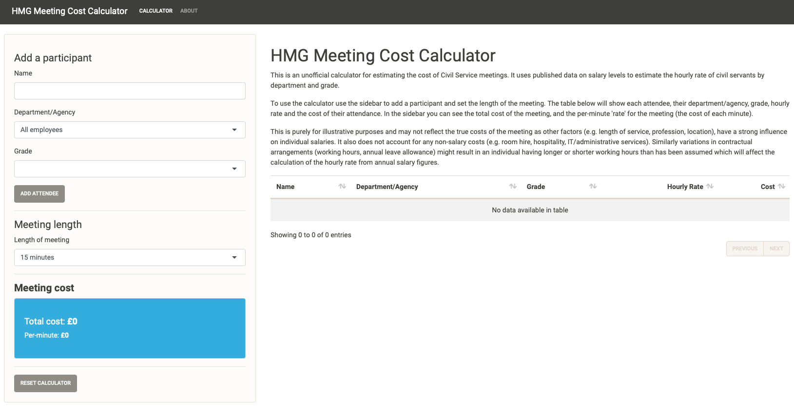
The user interface of the HMG Meeting Cost Calculator
We start off with an empty meeting - nobody is here so there’s no cost. So let’s add an attendee, we can give them a name, set their department/agency and their grade. Donna is a member of the Senior Civil Service (SCS) working in the Department for Digital, Culture, Media and Sport.
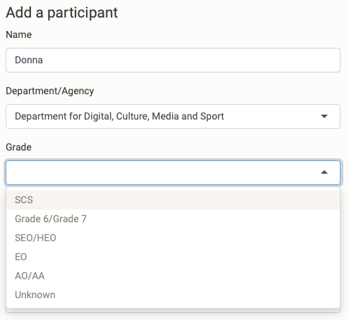
Providing Donna’s details
After we select the “Add attendee” button, her details are now added to the meeting. The default meeting length is the minimum setting (15 minutes), so we can already see that with Donna alone in this meeting the cost is £12.
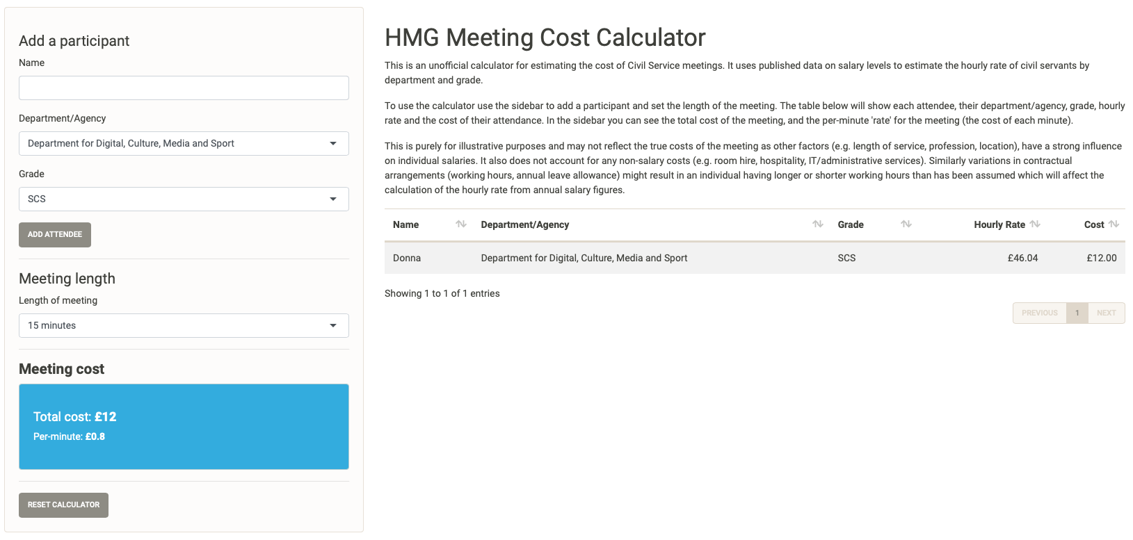
Donna’s meeting cost
Let’s add a couple of more colleagues from other departments and at other grades. Donna is joined by her colleague Dolly from the the Department of Health who is a Grade 6/Grade 7, as well as Agnetha a Grade 6/Grade 7 from the Foreign and Commonwealth Office who has brought along her assistant Anni-Frid who is an EO.

A multi-person meeting
We can now see that this 15 minute meeting of the four of them has an estimated cost of £33, or £2.20 per minute. While we might wish that many of the meetings we experience are just 15 minutes long, this one is actually going to last 1 hour and a half, so let’s update the meeting length. The price-per-minute doesn’t change, but the total cost of the meeting is now £198.20, we can also see the cost of each individual in the meeting is updated in the table.
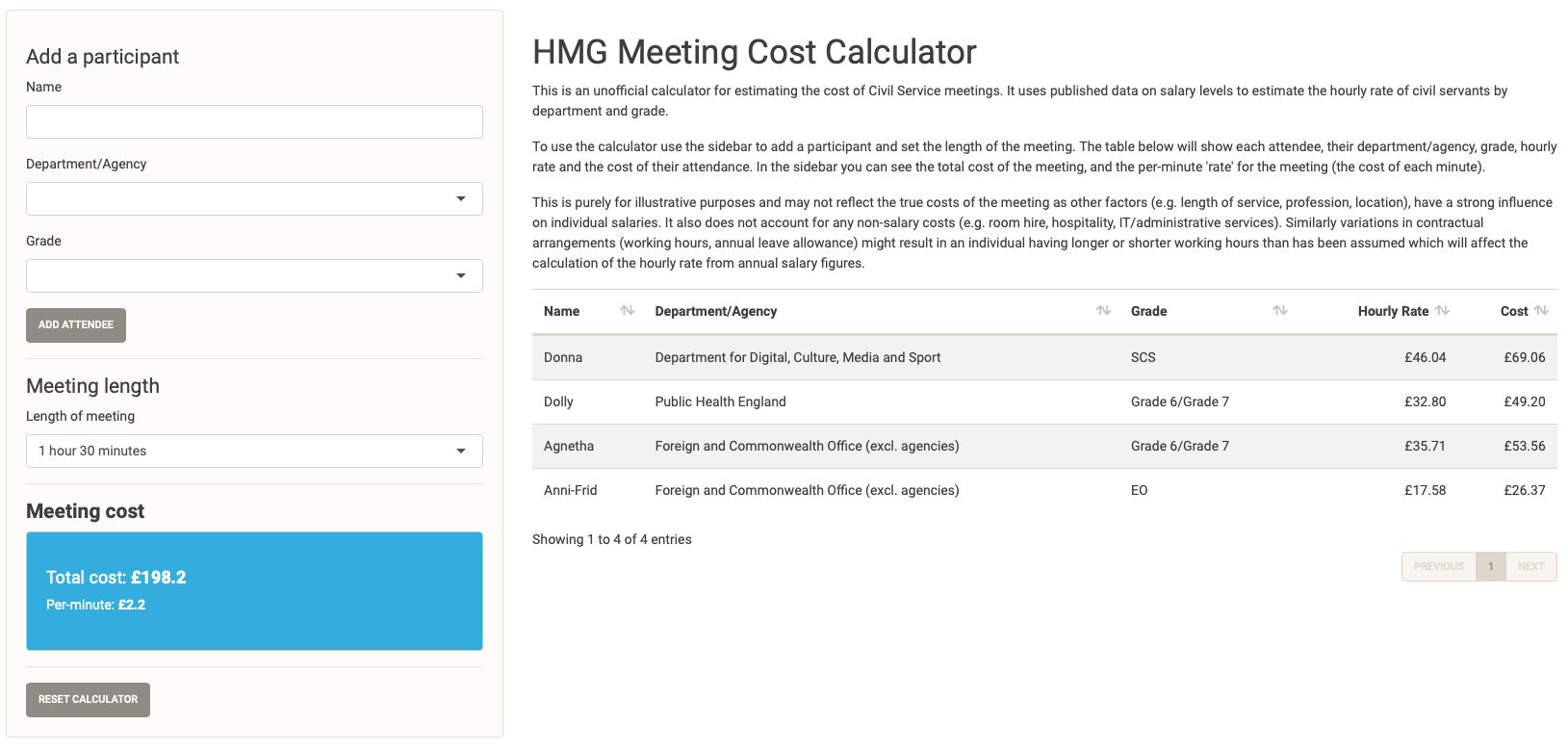
A ninety minute meeting
Despite its cost it’s decided that the meeting is very important needs to go ahead, but Donna realises that Beyonce an SCS at the Competition and Markets Authority also needs to attend and bring her colleagues Kelly and Michelle with her. The increases the per minute cost to £4.20, and the overall cost of the meeting to £378.20.
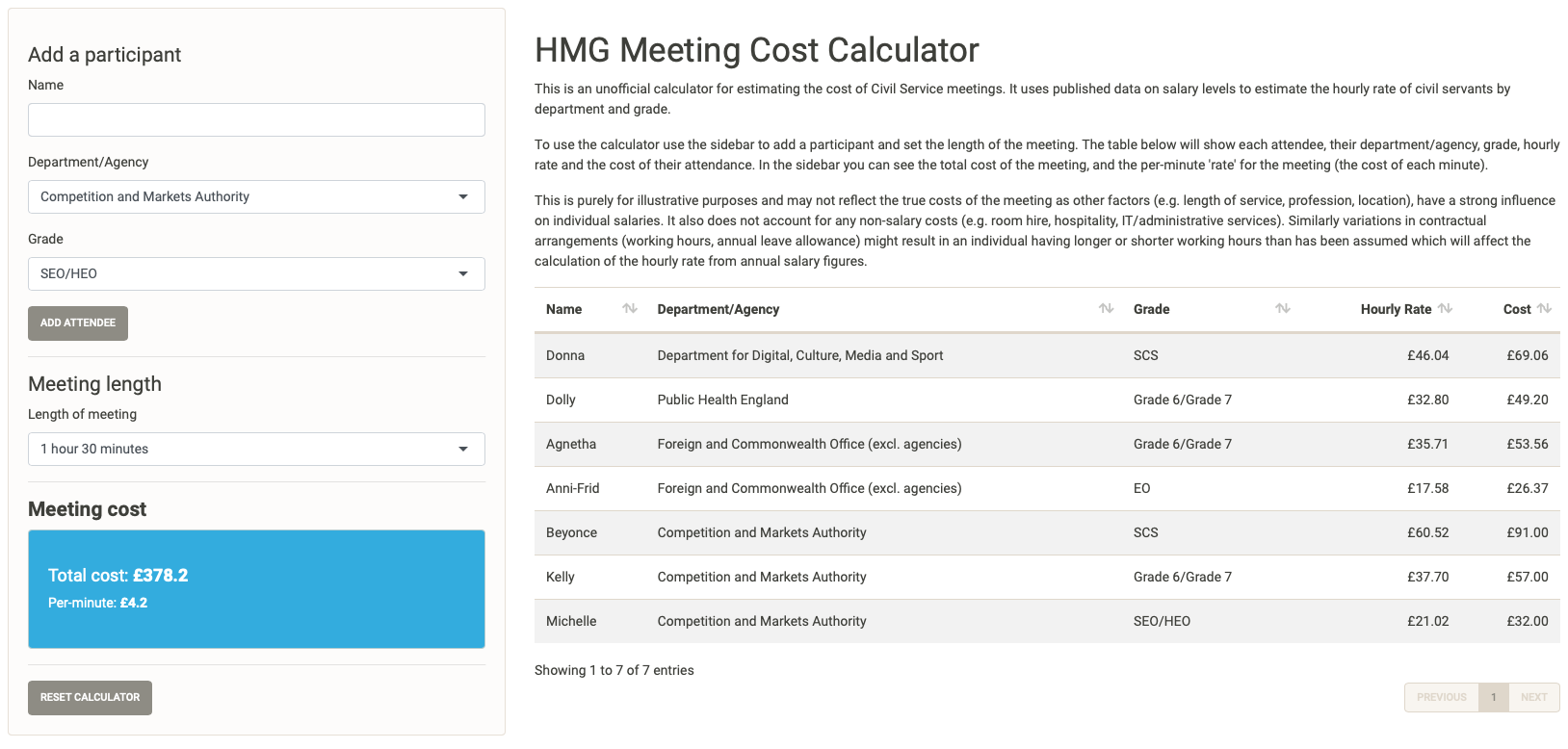
Even more attendees
Bills, Bills, Bills: under the hood of the app
There are several elements to the shiny server which we’ll consider in turn: storing the meeting data, capturing inputs and producing outputs.
Firstly, as we’re going to be using the inputs to add items to our dataset we need a way of storing the data we’ve previously input. We do this by creating a reactiveValues() object which stores values that can change. Let’s initalise our meeting this as an empty reactive object, and then let’s create within this an empty tibble that will hold our attendees, and a value for the total cost of the meeting.
meeting <- reactiveValues()

meeting$attendees <- tibble::tibble(
    name = character(),
    dept = character(),
    grade_label = character(),
    hourly_rate = numeric(),
    cost = numeric()
)

meeting$cost <- 0
Now after we’ve created the object we can write the code that responds to events in the UI. In addition to the fields to enter a name or select a department/grade/meeting length the UI also includes two buttons - one to add an attendee, and one to reset the table. We’ll write code so that the app only updates the meeting info when we choose to add an attendee, select a meeting time, or reset the table.
Let’s look at the add an attendee event first. Using observeEvent() we set the input element we want to ‘observe’ for action, and then supply a code block (using curly braces) that will be run when the add button is selected. When setting up our meeting object we didn’t collect the time, but we need this for our calculations so let’s take the information from the meeting length selector and store that as a numeric value. Then let’s create a tibble that contains the data of the attendee we want to add, so we need to collect their name, department, grade from the inputs. We can then use the department and grade to lookup the relevant hourly rate and join that to the attendee information. Finally we can calculate the cost of that individual attending the meeting by multiplying their hourly rate by the meeting time. Now that we have a tibble about the attendee we can add that to the existing meeting attendees tibble, we’ll also calculate the number of minutes the meeting is running for (the time is stored as hours) and update the total meeting cost as the sum of all the attendee costs). Finally we’ll reset the name field to empty so that the input is ready for a new attendee.
observeEvent(input$add, {

        meeting$time <- as.numeric(input$time)

        this_attendee <- tibble::tibble(
            name = input$name,
            dept = input$dept,
            grade_label = input$grade
        ) %>% left_join(salary_dept, by = c("dept", "grade_label")) %>%
            select(name, dept, grade_label, hourly_rate) %>%
            mutate(cost = janitor::round_half_up(hourly_rate * meeting$time))

        meeting$attendees <- bind_rows(meeting$attendees, this_attendee)
        meeting$minutes <- meeting$time * 60
        meeting$cost <- sum(meeting$attendees$cost)

        updateTextInput(session = getDefaultReactiveDomain(), inputId = "name", value = "")

    })
When the meeting length input is changed, we replace the meeting time value and the time in minutes value. We then recalculate the cost for each of the attendees and recalculate the total cost of the meeting.
observeEvent(input$time, {
        meeting$time <- as.numeric(input$time)
        meeting$minutes <- meeting$time * 60
        meeting$attendees$cost <- meeting$attendees$hourly_rate * meeting$time
        meeting$cost <- sum(meeting$attendees$cost)
    })
Finally, the reset button will reset the elements of reactive meeting object back to their defaults (i.e. an empty tibble of meeting attendees, total cost to 0), it will also reset the name, department, grade and meeting time inputs.
observeEvent(input$reset, {

        meeting$attendees <- tibble::tibble(
            name = character(),
            dept = character(),
            grade_label = character(),
            hourly_rate = numeric(),
            cost = numeric()
        )

        meeting$time <- as.numeric(input$time)
        meeting$minutes <- meeting$time * 60
        meeting$cost <- 0

        updateTextInput(session = getDefaultReactiveDomain(), inputId = "name", value = "")

        updateSelectInput(session = getDefaultReactiveDomain(), inputId = "dept", selected =  "All employees")

        updateSelectInput(session = getDefaultReactiveDomain(), inputId = "grade", selected = "")

        updateSelectInput(session = getDefaultReactiveDomain(), inputId = "time", selected = 0.25)


    })
Now let’s produce outputs to display in the Shiny app. To make the attendee table sortable we’ll use a {DT} datatable, which includes a renderDT() function that allows us to display interactive tables in our output. We use the attendees tibble from our meeting object, providing some human readable column names and formatting the final two columns as currency. We also want to provide the overall cost and cost per minute which we will pass back as rendered text, the per minute cost being calculated here by dividing the total cost by the number of minutes.
output$attendees <- DT::renderDT(
  DT::datatable(meeting$attendees,
  rownames = FALSE,
  colnames = c("Name", "Department/Agency", "Grade", "Hourly Rate", "Cost"),
  options = list(pageLength = 20, dom = "tip")) %>%
      DT::formatCurrency(4:5, "£"))

output$cost <- renderText(paste0("£", janitor::round_half_up(meeting$cost, 2)))

output$cost_minute <- renderText(paste0("£", janitor::round_half_up(meeting$cost / meeting$minutes, 2)))
And there we have it, the unofficial HMG Meeting Cost calculator app is complete4. The full code is available on github.
-
DISCLAIMER: I am a civil servant that works in the department responsible for the publishing of the data used in this post. However, I am not directly involved in the collation or analysis of this data in my day job. The analysis and resulting app are an entirely personal project conducted outside of work in my own time using my own resources, it uses only published data/information. It is not and should not be considered an official work of either my employing department or the UK government. Similarly any and all opinions in this post are made in a personal capacity and are not a statement of official UK government policy. ↩︎
-
In the 2020 statistics, 16 of the 53 tables relate to information about pay or salary. ↩︎
-
Remember
rowSums()is a quick function to summarise a numeric matrix/data frame,is.na(x)returns a logical version ofxinforming us whether the position inxis a missing value. As R inherently treats logical values as 0 forFALSEand 1 forTRUEwe can quickly calculate the row-wise sum of missing values in a data frame. ↩︎ -
I’m assuming you’ve already worked out the very important things happening in our example meeting!
↩︎