In my last post I wrote about the process for scraping data from Google’s COVID-19 Community Mobility Reports. That post dealt with processing just one report, the one for the UK, but Google have published reports for around 130 countries and one for each of the 50 US states. So we could run the script 180 separate times to extract all the data, but we can easily extend our scripting to automate this process.
Adopting functional programming
At the heart of any automation in R is the writing of functions, which allow you to quickly and easily run the same code again and again, with the same or different parameters. If you’re new to writing functions, I strongly recommend watching Hadley Wickham’s talk “The Joy of Functional Programming (for Data Science)” and the Functions chapter of his and Garret Grolemund’s book “R for Data Science”.
Functional programming requires a post (of series of posts) of its own. But the key thing that we need to do first is to break down our approach into a clear set of steps, these steps act as the markers for how to chunk your code into functions. There are two stages to the PDF scraping: (i) getting the overall country-level data, and (ii) getting the sub-national data. So these each have their own function get_national_data(url) and get_subnational_data(url) that each take a single argument, a URL for a Google community mobility report. These functions use the code written to scrape a PDF and return the resulting tibble of data for the report at the URL they’ve been given.
This is the first stage of automation, while R makes it easy to run code stored in a script via the source() command, encapsulating the code in a function means you can easily call that command again and again. By writing these two sets of code as functions we can use an argument, url, to pass it different information each time we run the command – the URL of different reports.
In reality there are actually four PDF scraping functions, there in addition to the national functions there are also get_regional_data(url) and get_subregional_data(url). In addition to country-level reports, Google have also published a report for each of the 50 US states. The structure for these reports is very similar to the country-level PDFs, so the code for these is very similar, except that a further column region is added to the output. There’s also some additional coding required to extract the region identifier.
Scraping the report download page
So the PDF scraping has been “automated” to just four functions, which means for any given report we’re just using one or two lines of code to extract many lines of data. But how do we find out the URLs for the reports. We could visit the webpage and either download all the reports and write code to iterated over the filenames in a given directory, or we could also manually copy the link for each report into a script.
Alternatively, we can let R do the hard work for us again. The {rvest} package provides a useful suite of functions to interact with, and extract, information from webpages. Webpages are written in HTML, a structured markup language. It is this structure which {rvest} is going to interact with, so we need to explore and understand it.
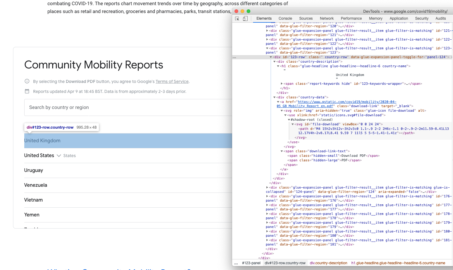
Screenshot of the download section of the Google COVID-19 Community Mobility Report webpage and its source code
While set out like a table, the download section is actually a set of <div> elements. To cut a long story structure short, the download links for each country are contained within a <div> element that has a class attribute of “country-data”, the links themselves use the standard HTML tag <a> which have the class attribute of “download-link”. The URLs are contained in the href attribute of the <a> tags.
url <- "https://www.google.com/covid19/mobility/"
page <- xml2::read_html(url)

country_urls <- page %>%
  rvest::html_nodes("div.country-data > a.download-link") %>%
  rvest::html_attr("href")
Before we can scrape the webpage we need to connect to it and read it, we do this by using xml2::read_html() and assign that to the object page so that we can easily refer to it in future. Then we need to identify the relevant “nodes” within the HTML that we are interested in, which we do passing a CSS selector to rvest::html_nodes(): div.country-data > a.download-link is asking for all nodes that are <a class="download-link"> tags inside of <div class="country-data"> elements. Having selected those nodes we can then extract the href attribute from the nodes using rvest::html_attr(). This returns a character vector of 131 URLs for the country-level PDF reports.
> country_urls
  [1] "https://www.gstatic.com/covid19/mobility/2020-04-05_AF_Mobility_Report_en.pdf"
  [2] "https://www.gstatic.com/covid19/mobility/2020-04-05_AO_Mobility_Report_en.pdf"
  [3] "https://www.gstatic.com/covid19/mobility/2020-04-05_AG_Mobility_Report_en.pdf"
  [4] "https://www.gstatic.com/covid19/mobility/2020-04-05_AR_Mobility_Report_en.pdf"
  [5] "https://www.gstatic.com/covid19/mobility/2020-04-05_AW_Mobility_Report_en.pdf"
We could just iterate our functions across this vector. However, it might be useful for us to have a record of these URLs and some other information associated with them.
country_list <- tibble(url = country_urls) %>%
  mutate(filename = basename(url),
         date = map_chr(filename, ~strsplit(., "_")[[1]][1]),
         country = map_chr(filename, ~strsplit(., "_")[[1]][2]),
         country_name = countrycode::countrycode(country,
                                                 "iso2c",
                                                 "country.name")) %>%
  select(country, country_name, date, url)
The filenames of the PDFs contain the date of the report and 2-character ISO country code for each country, so we can easily extract these to create a tibble that holds this information. We’re using purrr::map_chr() again to apply the strsplit() function to the filename and extract the relevant subsectios of the filename. Country codes aren’t something that everyone knows, so we can use the {countrycode} package to easily convert these into country names1. And now we have a nice simple tibble that gives us information about the country-level PDFs.
> country_list

|country |country_name      |date       |url                                                                           |
|:-------|:-----------------|:----------|:-----------------------------------------------------------------------------|
|AF      |Afghanistan       |2020-04-05 |https://www.gstatic.com/covid19/mobility/2020-04-05_AF_Mobility_Report_en.pdf |
|AO      |Angola            |2020-04-05 |https://www.gstatic.com/covid19/mobility/2020-04-05_AO_Mobility_Report_en.pdf |
|AG      |Antigua & Barbuda |2020-04-05 |https://www.gstatic.com/covid19/mobility/2020-04-05_AG_Mobility_Report_en.pdf |
|AR      |Argentina         |2020-04-05 |https://www.gstatic.com/covid19/mobility/2020-04-05_AR_Mobility_Report_en.pdf |
|AW      |Aruba             |2020-04-05 |https://www.gstatic.com/covid19/mobility/2020-04-05_AW_Mobility_Report_en.pdf |
We can use a similar process to get the URLs for all of the regional reports, using the CSS selector div.region-data > a.download-link.
region_urls <- page %>%
  rvest::html_nodes("div.region-data > a.download-link") %>%
  rvest::html_attr("href")

region_list <- tibble(url = region_urls) %>%
  mutate(filename = basename(url),
         date = map_chr(filename, ~strsplit(., "_")[[1]][1]),
         country = map_chr(filename, ~strsplit(., "_")[[1]][2]),
         region = map_chr(filename,
                          ~str_remove_all(., "-") %>%
                            str_remove("\\d+_\\w{2}_") %>%
                            str_remove("_Mobility_Report_en.pdf") %>%
                            str_replace_all("_", " "))) %>%
  select(country, region, date, url)
Extracting the region identifier from the filename is slightly more complex as the US states are in the filename by name rather than a code, so this is done by a nesting a series of stringr::str_remove and stringr::str_replace commands together. But ultimately we get a similar tibble to the country list.
> region_list

|country |region     |date       |url                                                                                      |
|:-------|:----------|:----------|:----------------------------------------------------------------------------------------|
|US      |Alabama    |2020-04-05 |https://www.gstatic.com/covid19/mobility/2020-04-05_US_Alabama_Mobility_Report_en.pdf    |
|US      |Alaska     |2020-04-05 |https://www.gstatic.com/covid19/mobility/2020-04-05_US_Alaska_Mobility_Report_en.pdf     |
|US      |Arizona    |2020-04-05 |https://www.gstatic.com/covid19/mobility/2020-04-05_US_Arizona_Mobility_Report_en.pdf    |
|US      |Arkansas   |2020-04-05 |https://www.gstatic.com/covid19/mobility/2020-04-05_US_Arkansas_Mobility_Report_en.pdf   |
|US      |California |2020-04-05 |https://www.gstatic.com/covid19/mobility/2020-04-05_US_California_Mobility_Report_en.pdf |
These two code blocks have also been converted into functions get_country_list() and get_region_list() respectively. You can specify a url as and argument, but they have a default argument of url=https://www.google.com/covid19/mobility/ to make it even easier for the user (and I suspect the main URL is unlikely to change).
Automating the extraction
Now that we’ve written our functions, and have a list of URLs, we can combine them together to automate the data extraction across all the reports.
country_list <- get_country_list()
region_list <- get_region_list()

country_dt <- country_list %>%
    mutate(overall_data = map(url, get_national_data),
           locality_data = map(url, get_subnational_data))

region_dt <- region_list %>%
    mutate(overall_data = map(url, get_region_data),
           locality_data = map(url, get_subregion_data))
This code gets the country and region lists, it then creates new tibbles taking and uses purrr::map() to apply the get_national_data() and get_subnational_data() (and their regional equivalents) to the URLs, these return columns that contain the tibbles output by each function.
> country_dt

|country |country_name      |region |date       |url         |overall_data    |locality_data    |
|:-------|:-----------------|:------|:----------|:-----------|:---------------|:----------------|
|AF      |Afghanistan       |NA     |2020-04-05 |https://... |<tibble [6 x 5]>|<tibble [0 x 5>  |
|AO      |Angola            |NA     |2020-04-05 |https://... |<tibble [6 x 5]>|<tibble [0 x 5>  |
|AG      |Antigua & Barbuda |NA     |2020-04-05 |https://... |<tibble [6 x 5]>|<tibble [0 x 5>  |
|AR      |Argentina         |NA     |2020-04-05 |https://... |<tibble [6 x 5]>|<tibble [144 x 5>|
|AW      |Aruba             |NA     |2020-04-05 |https://... |<tibble [6 x 5]>|<tibble [0 x 5>  |
We can expand these nested tibbles by using the purrr::map_dfr() function we used in the original PDF data extraction to merge these tibbles together. The data for at state-level for the US is duplicated (it’s the sub-national data in the US-level report and its the overall data extracted from each of the regional-level reports), the easiest way to programmatically de-duplicate the data was to US-level sub-national data as the region column.
countries_overall <- map_dfr(full_dt$overall_data, bind_rows)
locality_overall <- map_dfr(full_dt$locality_data, bind_rows) %>%
    filter(!(country == "US" & is.na(region)))

all_data_long <- countries_overall %>%
    bind_rows(locality_overall) %>%
    mutate(country_name = countrycode::countrycode(country, "iso2c", "country.name")) %>%
    select(date, country, country_name, region, location, entity, value)

  all_data_wide <- all_data_long %>%
    pivot_wider(names_from = entity, values_from = value)
Once combined the dataset is in a ’long’ format where there is a single datapoint on each row, however for analysis we probably want a ‘wide’ format where there is a single row per a geographic entity.
> all_data_wide %>% sample_n(5)

|date       |country |country_name   |region    |location                  | retail_recr| grocery_pharm| parks| transit| workplace| residential|
|:----------|:-------|:--------------|:---------|:-------------------------|-----------:|-------------:|-----:|-------:|---------:|-----------:|
|2020-04-05 |GB      |United Kingdom |NA        |Newry and Mourne and Down |       -0.86|         -0.41| -0.71|   -0.61|     -0.53|        0.30|
|2020-04-05 |JP      |Japan          |NA        |Oita                      |       -0.18|          0.03|  0.16|   -0.30|     -0.10|        0.06|
|2020-04-05 |FJ      |Fiji           |NA        |COUNTRY OVERALL           |       -0.52|         -0.33| -0.28|   -0.66|     -0.17|        0.18|
|2020-04-05 |US      |United States  |Indiana   |Shelby County             |       -0.49|         -0.14|    NA|   -0.47|     -0.35|        0.18|
|2020-04-05 |US      |United States  |Nevada    |REGION OVERALL            |       -0.49|         -0.22| -0.46|   -0.64|     -0.55|        0.15|
Automating the processing of the script
Having written functions to extract the data from both the webpage and the PDFs, and scripted the functions into a workflow we can easily run the script on demand to extract the data. However, we still need to run the script manually to extract the data. At present the code will also extract whatever is available on the website whether it’s been extracted before or not.
The master script has some additional features that allow it to be run automatically:
- The script automatically saves the
all_data_longandall_data_widetibbles as CSVs to thedatasubfolder including the report date in the filename. The script also appendscountry_listandregion_listto CSVs that store a record of what has been processed. - A function
get_update_time()scrapes the webpage for the metadata timestamp when the reports were updated. It will check this against the a timestamp stored in the repositoryLASTUPDATE_UTC.txt, which stores the last value of that metadata for reference purposes. If the timestamps match then the extraction code isn’t run. - If the reports have been updated but they have the same reference date the data is still extracted but warning is given to the user and the update timestamp is added to the exported files.
- A timestamp and message appended to the log file
processing.loggiving the outcome of the script (no update, existing reports updated, new reports published and extracted)
Using GitHub Actions to schedule the process
GitHub Actions is an automation facility built into GitHub, largely designed to provide continuous integration/deployment and testing for software packages. It is largely intended to be run when a commit is pushed to a repository (e.g. to build documentation, or test that new functionality works on multiple platforms). However, it can also be used to run scheduled jobs by making use of cron as an event trigger.
The base environments offered by GitHub do not include R, however the R community is rapidly developing mechanism to use GitHub Actions for R-based projects. It is already very easy to add R to a workflow through the r-lib/actions repository, and the {usethis} package has also been updated to provide easy to use functions for setting up GitHub Actions from within R. Based on GitHub’s own documentation and this ROpenSci playbook, I’ve developed a GitHub action workflow to run the get_all_data.R script on an hourly basis.
# Hourly scraping
name: googleC19scrape

# Controls when the action will run.
on:
  schedule:
    - cron: '0 * * * *'

jobs:
  autoscrape:
    # The type of runner that the job will run on
    runs-on: macos-latest

    # Load repo and install R
    steps:
    - uses: actions/checkout@master
    - uses: r-lib/actions/setup-r@master

    # Set-up R
    - name: Install packages
      run: |
        R -e 'install.packages("tidyverse")'
        R -e 'install.packages("pdftools")'
        R -e 'install.packages("countrycode")'
    # Run R script
    - name: Scrape
      run: Rscript get_all_data.R

    # Add new files in data folder, commit along with other modified files, push
    - name: Commit files
      run: |
        git config --local user.name github-actions
        git config --local user.email "actions@github.com"
        git add data/*
        git commit -am "GH ACTION Autorun $(date)"
        git push origin master
      env:
        REPO_KEY: ${{secrets.GITHUB_TOKEN}}
        username: github-actions
Firstly we define when the workflow runs, there are a large number of events that can trigger a workflow (e.g. when a push is made to a repository or a pull request intiated, a release is published), but we can also define a regular schedule using cron syntax. Next we define the environment we will run our script on (in this case macos-latest, there are also Ubuntu and Windows options available, and an action can also run in multiple environments). It then works through a series of steps, firstly loading the repository and installing R, install the necessary packages from CRAN and then running the actual R script for checking and extracting data. After the script is run we then commit any new files in the data folder and commit those along with any other files that have been modified (i.e. log files) and push these to the repository.
And now on an hourly basis the code will run and update the repository with new data.
-
{countrycode}is a rather fantastic package which will certainly be the subject of a future blog. ↩︎