Last week Google published their COVID-19 Community Mobility Reports. These make use of Google’s very extensive location history data, which they mainly use for telling you about traffic levels on roads, popular times for places in Google Maps and whether a bar or restaurant is busier than usual. In these mobility reports they’ve looked at the location history data for a large number of countries, and localities within countries to help public health officials review the effectiveness of social distancing measures.
Social distancing is one of the key non-medical interventions that governments have been putting in place to deal with the COVID-19 outbreak. So data about where people are/aren’t going is crucial to understanding the effectiveness of the social distancing measures that have been put in place. Full credit to Google for putting their data to good use and providing public health officials and governments with analysis they can use in policy-making.
But… the data has been published in PDF format, so while this makes it easy to view at a glance it’s not that easy to reuse or plug into other things. To be honest, I’m quite surprised it’s not also available in a spreadsheet of some sort of machine-readable format.
So, last Friday I set out to write some code to scrape the reports. Initially this was just to get the data from the UK report, but as the PDFs have a standardised format it can be, and was, easily applied to the reports for all countries and US states. You can view and download the code yourself from this GitHub repo.
Getting started
First off, I’m by no means an expert at web/PDF scraping, all I’ve learnt about it I’ve learnt-by-doing. My code is simply extracting the headline comparison figures that are written in the reports. Colleagues at the ONS’ Data Science Campus have done an excellent job and have developed a tool to extract the trend-line data from the reports. Duncan Garmonsway has then ported the ONS code to R. Even so, I’m sure the headline figures are still useful to have, especially if you want to compare several areas at once.
We could just download the relevant PDF, i.e. the UK one, and transpose the numbers by hand to a spreadsheet: (a) that sounds like a really fun job!!; (b) especially if they update the reports; and, (c) it wouldn’t make much of a blog post.
To start with I did download the UK PDF in order to explore its structure, but I quickly changed even that initial scripting to work from the URL of the PDF. I then went about automating the process to extract the data for all PDFs and then to handle the PDFs being updated on a regular basis. This post sets out the approach to scraping a single PDF report, a future post will describe the approach to automating this for all reports.
PDF scraping
Scraping the PDFs is done using the {pdftools} package from ROpenSci. This is a really good and easy to use package for working with PDFs in R. The code uses pdftools::pdf_data() to extract the data, which is a rather amazing function.
url <- "https://www.gstatic.com/covid19/mobility/2020-04-05_GB_Mobility_Report_en.pdf"
report_data <- pdftools::pdf_data(url)
This code gives us report_data, which is a list of tibbles where each tibble represents a single page of the PDF and each tibble contains data about all of the text on that page. So report_data[[2]] is the data about all the text elements of page 2 of the PDF.
The tibble for page 2 of the UK’s PDF looks like this:
> report_data[[2]]

| width| height|   x|   y|space |text     |
|-----:|------:|---:|---:|:-----|:--------|
|    33|     13|  36|  36|TRUE  |Transit  |
|    39|     13|  72|  36|FALSE |stations |
|    17|      7| 167|  49|FALSE |+80%     |
|    89|     45|  36|  62|FALSE |-70%     |
|    36|      9|  36| 116|TRUE  |compared |
width and height are the size in pixels of the text box that the piece of text is contained in, x and y is the pixel position of the top left corner of the text box, space indicates whether there is a space after the text, and text is the actual text. So what we’re getting from pdftools::pdf_data() is a reference object about every single bit of text in a PDF.
But before we go any further we need to think about the structure of the PDFs. The first two pages are the overall data for that country, then all the other pages except the last page are for sub-national locations, and the last page briefly describes the data and the report. While the reports contain the same six sets of data for the national and sub-national areas, the national data is spread over two pages while the sub-national data is displayed two areas to a page. So it makes sense to run these as two separate processes, and they have ended up as two separate functions in my code: get_national_data() and get_subnational_data().
National data
With the national data being spread over two pages this means that its in two separate elements of the report_data list. The code extracts and combines the tibbles for pages 1 and 2 as follows:
national_pages <- report_data[1:2]
national_data <- purrr::map_dfr(national_pages, dplyr::bind_rows, .id = "page")
The {purrr} package is designed to make it much easier to work with lists, purrr::map_dfr() takes a list, applies a function to that list and returns (as the dfr part of the name suggests) a set of data frame rows. This code snippet is taking the first two elements of the report_data list and using dplyr::bind_rows() to combine them together into a single table. The code also uses the argument .id = page to add a column called page to the output tibble so that we know which page of the PDF the item of text has come from. Technically its just calling the index number from the list, but in this example this neatly marries up with the actual pages in the PDF.
Now we have a single tibble that contains all the data we need to extract. So let’s do that.
national_datapoints <- national_data %>%
  filter(y == 369 | y == 486 | y == 603 |
         y == 62  | y == 179 | y == 296) %>%
  mutate(
    entity = case_when(
      page == 1 & y == 369 ~ "retail_recr",
      page == 1 & y == 486 ~ "grocery_pharm",
      page == 1 & y == 603 ~ "parks",
      page == 2 & y == 62  ~ "transit",
      page == 2 & y == 179 ~ "workplace",
      page == 2 & y == 296 ~ "residential",
      TRUE ~ NA_character_)) %>%
  mutate(value = as.numeric(str_remove_all(text, "\\%"))/100,
         date = date,
         country = country,
         location = "COUNTRY OVERALL") %>%
  select(date, country, location, entity, value)
Inspecting national_data tibble I was able to find x,y coordinates of each of the percentages for the six sets of location history data contained in the reports. I also discovered that they had a unique y-coordinates, no other text entity shared a y-coordinate with the percentages. So we can filter the tibble to provide the table rows that match those y-coordinates. Job done? Not quite.
While we could use the code to also locate the labels for these entities, given that we know the page and y position of these entities, we can use dplyr::case_when() to easily assign each row an entity label based on those attributes. This also ensures that we’ve got consistent names in our tables. Finally we need to convert the percentages to a numeric value, which we do by removing the percent sign and dividing by 100. The code also adds the date of the report and the country code, both of which are extracted from the PDF file name. Finally, for working with a merged dataset of national and sub-national data a location column is added, but in this case it’s set to “COUNTRY OVERALL”.
And now we have a nice simple tibble, national_datapoints, that contains the national percentages from the UK’s mobility report.
> national_datapoints

|date       |country |location        |entity        | value|
|:----------|:-------|:---------------|:-------------|-----:|
|2020-04-05 |GB      |COUNTRY OVERALL |retail_recr   | -0.82|
|2020-04-05 |GB      |COUNTRY OVERALL |grocery_pharm | -0.41|
|2020-04-05 |GB      |COUNTRY OVERALL |parks         | -0.29|
|2020-04-05 |GB      |COUNTRY OVERALL |transit       | -0.70|
|2020-04-05 |GB      |COUNTRY OVERALL |workplace     | -0.54|
|2020-04-05 |GB      |COUNTRY OVERALL |residential   |  0.15|
Sub-national data
The sub-national data for the UK is included at page 3 until page 77, however to make the code suitable for running on any PDF let’s subset report_data dynamically to the penultimate page, which we can do by getting the length() of report_data and subtracting one from it. As with the national data let’s pass this through purrr::map_dfr() to create a single tibble of all sub-national text entities.
subnational_pages <- report_data[3:(length(report_data)-1)]
subnational_data <- map_dfr(subnational_pages, bind_rows, .id = "page")
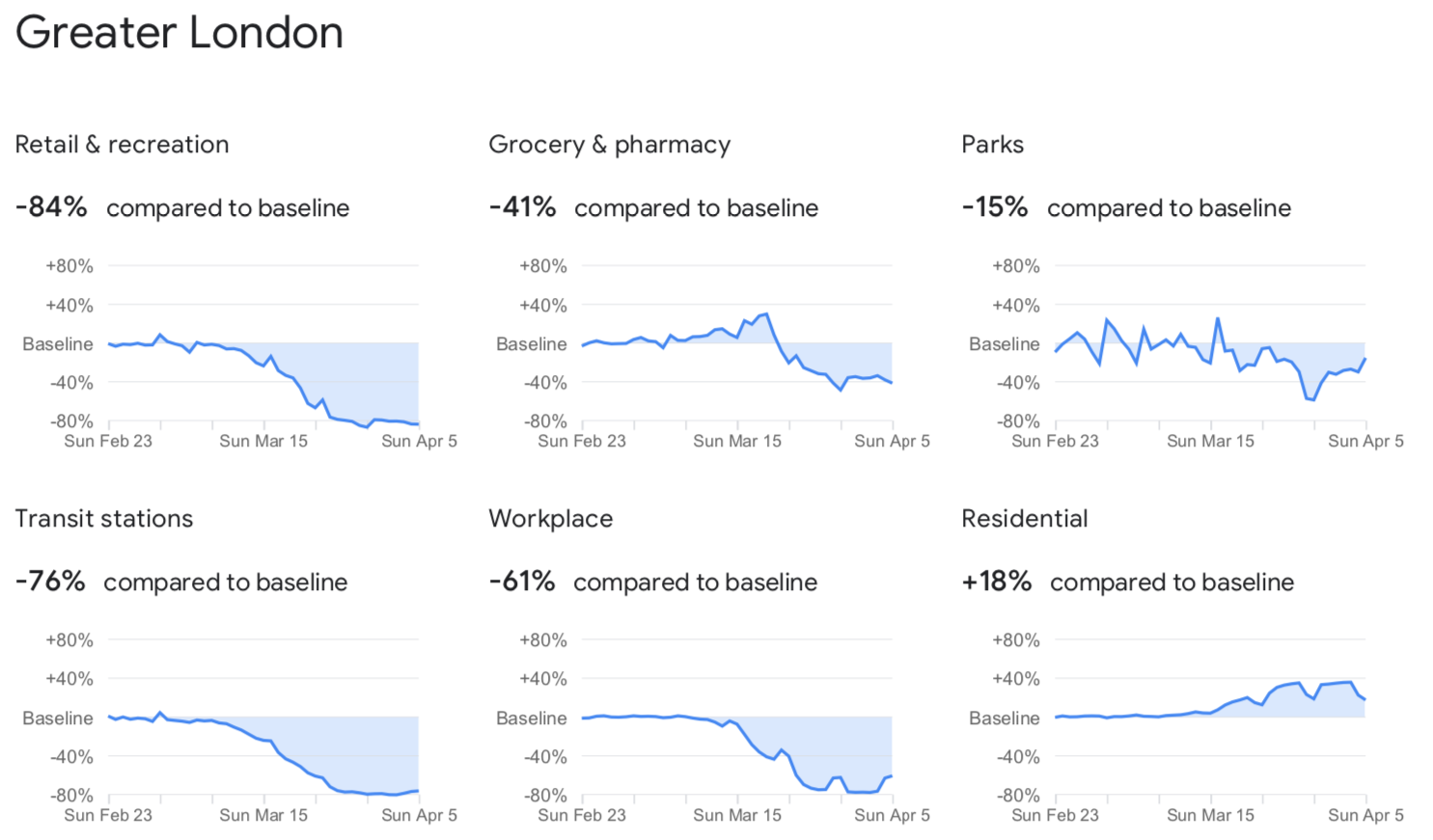
So far, so similar; but now it gets more complex. The cover image for this post is the set of charts for Greater London from the 5th April 2020 report, can you guess what the complexities are?

Well, the complexities are:
- We need to capture the location name, not just the figure
- For each location the data is arranged in two rows of three charts each
- There is data for two locations per page
Again, in inspecting subnational_data it was possible to identify that locations and the percentages had common x,y coordinates on each page. So we can easily extract them by filtering the tibble just as we did for the national data.
subnational_datapoints <- subnational_data %>%
  filter(y == 36  | y == 104 | y == 242 |
         y == 363 | y == 431 | y == 568) %>%
  mutate(
    entity = case_when(
      y == 36 ~ "location",
      y == 104 & x == 36  ~ "retail_recr",
      y == 104 & x == 210 ~ "grocery_pharm",
      y == 104 & x == 384 ~ "parks",
      y == 242 & x == 36  ~ "transit",
      y == 242 & x == 210 ~ "workplace",
      y == 242 & x == 384 ~ "residential",
      y == 363 ~ "location",
      y == 431 & x == 36  ~ "retail_recr",
      y == 431 & x == 210 ~ "grocery_pharm",
      y == 431 & x == 384 ~ "parks",
      y == 568 & x == 36  ~ "transit",
      y == 568 & x == 210 ~ "workplace",
      y == 568 & x == 384 ~ "residential"),
    position = case_when(
      y == 36 ~ "first",
      y == 104 ~ "first",
      y == 242 ~ "first",
      y == 363 ~ "second",
      y == 431 ~ "second",
      y == 568 ~ "second")
  )
Having inspected the PDFs, for each location there are just three lines we need to concern ourselves with: the location, the first row of percentages and the second row of percentages. As there are two locations to a page we end up with six y positions that we care about. So we can filter the dataset down to just the rows where y matches one of these six positions.
Again we can use dplyr::case_when() to label each of these entities, which we can do using matching their coordinates to the x and y columns in the tibble. The location name is the only entity on its respective y-coordinate so we can do away matching the x-coordinate, actually we definitely shouldn’t match on the x-coordinate but more on that later. For the six percentages we need both the x and y, and again these are standardised not only across pages but also with page such that the x position for parks is always 384 whether it is in the upper or lower set of graphs. We also record whether the data is for the first or second location on a page.
Most of the sub-national locations in the UK report (and those of other countries) have more than one word in their name. pdftools::pdf_data() treats each word as a separate entity, and so appears as a separate row in the resulting tibble(s). This is why we didn’t match the location label to a given x-coordinate, so that we can pick up all of the words used to describe locations.
> subnational_datapoints

|page | width| height|   x|   y|space |text          |entity   |position |
|:----|-----:|------:|---:|---:|:-----|:-------------|:--------|:--------|
|1    |    75|     20|  36|  36|TRUE  |Aberdeen      |location |first    |
|1    |    30|     20| 115|  36|FALSE |City          |location |first    |
|1    |   112|     20|  36| 363|FALSE |Aberdeenshire |location |second   |
|2    |    47|     20|  36|  36|TRUE  |Angus         |location |first    |
|2    |    54|     20|  87|  36|FALSE |council       |location |first    |
|2    |    51|     20|  36| 363|TRUE  |Antrim        |location |second   |
|2    |    30|     20|  91| 363|TRUE  |And           |location |second   |
|2    |   120|     20| 126| 363|FALSE |Newtownabbey  |location |second   |
This is the location data from the first two sub-national pages, only one of the four locations has a single word name, Aberdeenshire, the other three are multi-word names: Aberdeen City; Angus council; Antrim And Newtownabbey. So how do we combine these together? Our friend the {purrr} package is back to the rescue, this time though purrr::map_chr() which outputs a character vector.
locations <- subnational_datapoints %>%
  filter(entity == "location") %>%
  select(page, position, text) %>%
  group_by(page, position) %>%
  nest() %>%
  mutate(location = map_chr(data, paste),
         location = str_remove_all(location, "^c\\(\""),
         location = str_replace_all(location, "\", \"", " "),
         location = str_remove_all(location, "\"\\)"),
         location = str_replace_all(location, "And", "and")) %>%
  select(page, position, location)
First we filter the subnational_datapoints tibble to just the location entities, and then we take just the page, position and text columns. Using dplyr::group_by() and tidyr::nest() we convert the tibble into a “grouped data frame”, so the main tibble is now one row per page and position with a column called data that contains a tibble in each row of the other columns from the original tibble. In this case these per-page-position tibbles are just a single column, text. We can now apply purrr::map_chr() to this data column to work with all the information in each nested tibble. As we want to stitch the words together we can just use paste(). The resulting character string is a bit messy so the code runs a series of stringr::str_remove_all() and stringr::str_replace_all() commands to simplify into a label. Finally, let’s select just the page, position and new location columns, and now we have a list of locations that we can merge with our data.
location_data <- subnational_datapoints %>%
  left_join(locations, by = c("page", "position")) %>%
  filter(entity != "location") %>%
  mutate(value = as.numeric(str_remove_all(text, "\\%"))/100,
         date = date,
         country = country) %>%
  select(date, country, location, entity, value)
Using dplyr::left_join() we can merge our new location labels with the extracted data using the page and position as the matching keys. Now that we’ve got nice location labels attached to the data we can drop the rows relating to the location entity. As with the national data we convert the percentages to a value and add the data and country from the file name. This gives us a ’long’ tibble of all the data points by location.
> location_data

|date       |country |location                |entity        | value|
|:----------|:-------|:-----------------------|:-------------|-----:|
|2020-04-05 |GB      |Aberdeen City           |retail_recr   | -0.84|
|2020-04-05 |GB      |Aberdeen City           |grocery_pharm | -0.37|
|2020-04-05 |GB      |Aberdeen City           |parks         | -0.39|
|2020-04-05 |GB      |Aberdeen City           |transit       | -0.71|
|2020-04-05 |GB      |Aberdeen City           |workplace     | -0.57|
|2020-04-05 |GB      |Aberdeen City           |residential   |  0.30|
Depending on our uses it might be better to turn this into wide format using tidyr::pivot_wider().
> location_data %>% pivot_wider(names_from = "entity", values_from = "value")

|date       |country |location                | retail_recr| grocery_pharm| parks| transit| workplace| residential|
|:----------|:-------|:-----------------------|-----------:|-------------:|-----:|-------:|---------:|-----------:|
|2020-04-05 |GB      |Aberdeen City           |       -0.84|         -0.37| -0.39|   -0.71|     -0.57|        0.30|
|2020-04-05 |GB      |Aberdeenshire           |       -0.76|         -0.44| -0.35|   -0.55|     -0.51|        0.27|
|2020-04-05 |GB      |Angus council           |       -0.79|         -0.41| -0.28|   -0.43|     -0.48|        0.20|
|2020-04-05 |GB      |Antrim and Newtownabbey |       -0.79|         -0.47| -0.70|   -0.89|     -0.53|        0.30|
|2020-04-05 |GB      |Ards and North Down     |       -0.76|         -0.37| -0.59|   -0.53|     -0.56|        0.29|
And there you have it, Google’s COVID19 Community Mobility Data for 150 UK locations in a nice easy to reuse table. If you want to run the code yourself, or download the data, visit this GitHub repo. In a future blog I’ll write about automating this to run over all of the published PDFs