Energy costs in the UK, and globally, have been rising significantly as a result of Russia’s invasion of Ukraine. Energy prices for domestic (i.e. residential/household) consumers in the UK have been subject to a “cap”1 calculated by the energy regulator, Ofgem. The price cap is usually quoted in terms of it’s annual value, which possibly isn’t the most useful approach, especially as we head into the winter months. So I tried to estimate what my energy costs might be… and then I turned that exercise into an interactive calculator that others can use.
Let’s get the rant out of the way2
Ugh. Just ugh. The energy price crisis isn’t just a “crisis”, it’s a hellish nightmare. It’s multifaceted and it feels like at every step the government is determined to do the bare minimum3. But, in addition to the any short-term intervention its also a demonstration of the fundamental problem at heart of government by the Conservatives since 2010, a failure of long-term strategic thinking. Under the branding of austerity, various energy infrastructure and incentive programmes where cancelled in the 2010s. Much of our gas storage capacity was deemed unnecessary and sold off. The UK has some of the worst insulated homes in Europe. Our electricity market is still heavily linked to gas; even if you have a 100% green electricity tariff/supplier, your price is still determined by the gas prices. And then you come to the here and now, where even with a windfall tax energy companies are making record profits, small businesses are closing due to their uncapped costs, families that are already dealing with a near doubling of energy prices in the past year are struggling to pay bills. The government has committed to paying something, but this was months ago and the changing wholesale costs mean its relative impact is diminishing rapidly. Meanwhile, there are siren noises circling around the government to “cut the green crap” that (a) won’t actually have much impact on bills and (b) will further exacerbate our problematic reliance on fossil fuels, which is part of the reason we’re in this crisis in the first place.
How much energy do I use over the year?
Amidst that background of horror, I made the decision this summer to quit my job and become a freelancer. The never ending cycle of news about price rises, especially energy has me worried. I’ve already had my monthly direct debit double last October, and who knows what it’ll be. “Three and a half thousand”, “four thousand”, “six thousand”, these are big numbers bandied about when government and the media talk about energy prices. But they’re illusions. Firstly, they come from headline figures in Ofgem’s model which uses a specific level of energy consumption that is claimed to represent the average household. Moreover, most (if not all) households pay for energy much more frequently than on an annual basis, which given that the price cap is now going to change quarterly makes an annual estimate a bit of problem. Especially as we move into the winter months.
I have a smart meter for both my electricity and gas and every half an hour they send my energy company information about my consumption. In theory there’s information out there about my energy usage since they were installed in July 2017, in practice its more complicated. I switched suppliers in 2020, and so I don’t have access to the data from my previous supplier, my current supplier has an API that I can pull data from, but for some reason it only takes me back to the start of 2022. So, relying on actual data is out of the window4. But I could take my annual consumption figures, which I can get from my latest energy bill, and use a national average to estimate how that figure changes over the course of the year.
How much does energy usage change month-on-month
The UK government produces volumes and volumes of data about energy statistics, so surely there’s a nice simple table of monthly domestic electricity and gas consumption, ideally by household type. No5. So let’s just use overall gas and electricity consumption as a proxy. These are available in Energy Trends table 4.2 for gas and table 5.5 for electricity6.
First lets just extract the relevant columns from each spreadsheet. For gas we’ll take the “Gas output from transmission” column, which is the gas supplied to end customers. For electricity we’ll take the “Total electricity consumption” which is energy used by end customers.
et_42_gas <- readxl::read_excel(
  path = "data/ET_4.2_AUG_22.xlsx",
  sheet = "Month (GWh)"
)

et_55_elec <- readxl::read_excel(
  path = "data/ET_5.5_AUG_22.xlsx",
  sheet = "Month"
)

gas_output <- et_42_gas[7:nrow(et_42_gas), c(1, 17)]
names(gas_output) <- c("ref_month", "gas_gwh")
# correct double space in November 2006 label
gas_output <- gas_output |>
  dplyr::mutate(ref_month = stringr::str_replace(ref_month, "  ", " "))

elec_consumption <- et_55_elec[6:nrow(et_55_elec), c(1, 16)]
names(elec_consumption) <- c("ref_month", "elec_twh")
> gas_output
# A tibble: 318 × 2
   ref_month      gas_gwh
   <chr>          <chr>
 1 January 1996   106090
 2 February 1996  106122
 3 March 1996     99942
 4 April 1996     71287
 5 May 1996       67630

> elec_consumption
# A tibble: 330 × 2
   ref_month      elec_twh
   <chr>          <chr>
 1 January 1995   26.98
 2 February 1995  26.5
 3 March 1995     31.691800000000001
 4 April 1995     22.85
 5 May 1995       21.7
Next let’s calculate the relative monthly energy consumption. Let’s join our two datasets, convert the columns from character vectors to date and numeric vectors, and extract month and year components from the date. Let’s limit ourselves to more recent data, but not the current calendar year as data could still be revised. Then for each fuel and calendar year let’s calculate the monthly consumption relative to the highest monthly consumption.
energy_trends <- elec_consumption |>
  dplyr::full_join(gas_output, by = "ref_month") |>
  dplyr::mutate(
    ref_month = lubridate::my(ref_month),
    month = lubridate::month(ref_month),
    year = lubridate::year(ref_month),
    across(c(elec_twh, gas_gwh), as.numeric)
  ) |>
  tidyr::pivot_longer(cols = c(elec_twh, gas_gwh), names_to = "fuel",
                      values_to = "consumption") |>
  dplyr::mutate(fuel = if_else(fuel == "elec_twh", "electricity", "gas")) |>
  dplyr::filter(year >= 2010 & year < 2022) |>
  dplyr::group_by(fuel, year) |>
  dplyr::mutate(
    # calculate relative trend
    relative_value = consumption / max(consumption)
  ) |>
  dplyr::ungroup()
This shows us that while there are, inevitably, differences between years there is a relatively consistent pattern in monthly energy consumption. For electricity we see only a small dip in relative consumption, in summer months the UK consumes around 80% of the electricity of winter months. For gas we see a much more pronounced variation in usage, with usage in summer months around 40% of winter consumption. So it’s probably quite critical if we’re thinking about what a price cap means in practice to consider this monthly pattern of energy usage, especially as by the time of the potential £6,600 cap in April gas usage will start to drop.
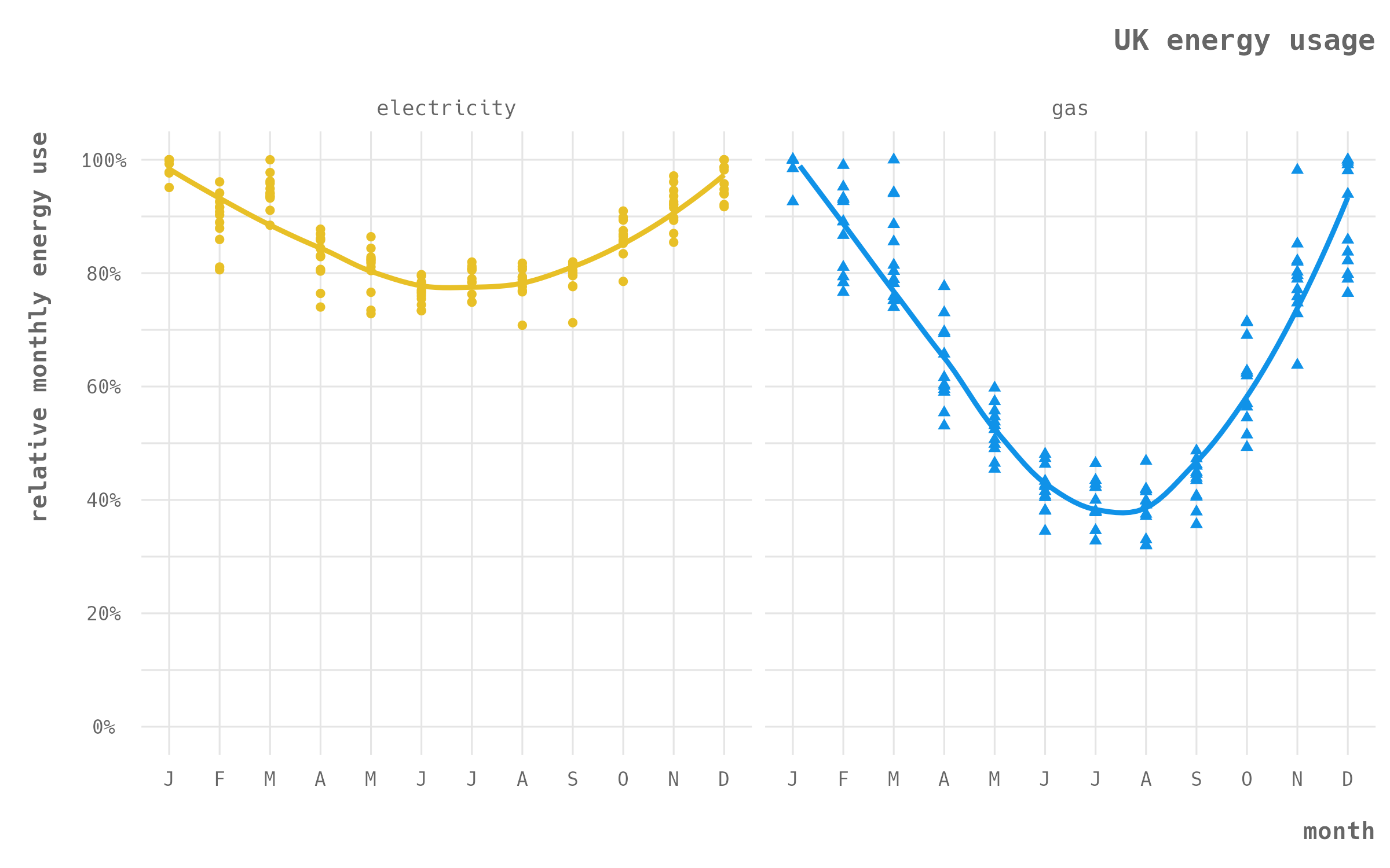
UK energy trends
Plot code
ggplot(energy_trends_gdt, aes(x = month, y = value, colour = fuel,
                              shape = fuel)) +
  geom_point() +
  geom_smooth(se = FALSE) +
  # geom_line(data = energy_trend_summary, colour = "grey40", linetype = "dashed") +
  facet_wrap(~fuel, nrow = 1) +
  scale_y_continuous(limits = c(0, 1), breaks = seq(0, 1, 0.2), labels = scales::percent_format()) +
  scale_x_continuous(
    breaks = 1:12,
    labels = c("J", "F", "M", "A", "M", "J", "J", "A", "S", "O", "N", "D")
  ) +
  scale_color_manual(values = energy_colours) +
  labs(
    title = "UK energy usage",
    y = "relative monthly energy use"
  ) +
  mattR::theme_lpsdgeog() +
  theme(
    panel.grid.minor.x = element_blank(),
    legend.position = "none"
  )
Having got monthly relative figures let’s calculate the average for each month, we also need to convert this to a proportion so that we can take an annual figure and estimate the gas usage for a given month.
energy_trend_summary <- energy_trends |>
  dplyr::select(month, fuel, relative_value) |>
  dplyr::group_by(fuel, month) |>
  dplyr::summarise(value = mean(relative_value), .groups = "drop_last") |>
  dplyr::mutate(
    value = value/max(value),
    prop = value/sum(value)
  )
> energy_trend_summary |> arrange(month, fuel)
# A tibble: 24 × 4
# Groups:   fuel [2]
   fuel        month value   prop
   <chr>       <dbl> <dbl>  <dbl>
 1 electricity     1 1     0.0959
 2 gas             1 1     0.127
 3 electricity     2 0.901 0.0864
 4 gas             2 0.885 0.112
So what’s it going to cost?
Now that we have a way of estimating usage we need to figure out a way to estimate the costs. First let’s set up a tibble with the values of the price cap for the coming months. We’ll be using the Cornwall Insight figures of £5,387, £6,616 and £5,897 for January to September 2023, these are the annual figures for a dual fuel direct debit customer. Based on the Ofgem price cap model we can estimate that the dual fuel cost is weighed approximately 51.3% gas and 48.7% electricity. The Ofgem model provides us with a split of the electricity and gas figures, so we can use these for October to December 2022. The price cap headlines are also based on an “average” consumption of 3,100 kWh of electricity and 12,000 kWh of gas, so we can divide our figures by this amount to get a price per kilowatt-hour. For simplicity of the future calculations the Ofgem daily standing charges have been added to the fuel totals.
cap_estimates <- tibble::tibble(
  month = c(10:12, 1:3, 4:6, 7:9),
  cap_forecast = c(rep(NA_real_, 3), rep(5387, 3), rep(6616, 3), rep(5897, 3)),
  electricity = 0.487 * cap_forecast / 3100,
  gas = 0.513 * cap_forecast / 12000
) |>
  mutate(
    electricity = if_else(month %in% 10:12, (1778 + 169) / 3100, electricity),
    gas = if_else(month %in% 10:12, (1875 + 104) / 12000, gas)
  )
> cap_estimates
# A tibble: 12 × 4
   month cap_forecast electricity   gas
   <int>        <dbl>       <dbl> <dbl>
 1    10           NA       0.628 0.165
 2    11           NA       0.628 0.165
 3    12           NA       0.628 0.165
 4     1         5387       0.846 0.230
 5     2         5387       0.846 0.230
 6     3         5387       0.846 0.230
 7     4         6616       1.04  0.283
 8     5         6616       1.04  0.283
 9     6         6616       1.04  0.283
10     7         5897       0.926 0.252
11     8         5897       0.926 0.252
12     9         5897       0.926 0.252
So we’re ready to simulate some costs. First we need to simulate the months of the year starting in October 2022 and working our way through to September 2023. Now we can merge in the usage figures from our analysis of Energy Trends and then merge in the price cap estimates. Then we simulate usage, let’s use the default consumption from the Ofgem price cap of 3,100 kWh for electricity and 8,200 for gas, and we multiply them by the monthly fuel proportion value. Finally, we can multiply these usage estimates with the price cap to simulate the likely month-by-month costs.
cost_simulator <- tibble::tibble(
  # set-up simulator for Oct 2022 to September 2023
  year = rep(c(rep(2022, 3), rep(2023, 9)), 2),
  month = rep(c(10:12, 1:9), 2),
  fuel = sort(rep(c("electricity", "gas"), 12))
) |>
  dplyr::left_join(
    # merge monthly usage proportion
    energy_trend_summary, by = c("month", "fuel")
  ) |>
  dplyr::left_join(
    # merge kwh cost estimates
    cap_estimates |>
      dplyr::select(-cap_forecast) |>
      tidyr::pivot_longer(cols = -month, names_to = "fuel",
                          values_to = "cap"),
    by = c("month", "fuel")
  ) |>
  dplyr::mutate(
    # estimate usage for default
    default_usage = if_else(
      fuel == "electricity",
      prop * 3100,
      prop * 12000
    ),
    # estimate cost for default
    default_cost = cap * default_usage,
  )

month_totals <- cost_simulator |>
  dplyr::select(ref_month, fuel, default_cost) |>
  tidyr::pivot_wider(names_from = fuel, values_from = default_cost) |>
  dplyr::mutate(
    total = electricity + gas
  )
> month_totals
# A tibble: 12 × 4
   ref_month  electricity   gas total
   <date>           <dbl> <dbl> <dbl>
 1 2022-10-01        162.  154.  317.
 2 2022-11-01        173.  201.  374.
 3 2022-12-01        182.  228.  410.
 4 2023-01-01        252.  351.  603.
 5 2023-02-01        227.  311.  538.
 6 2023-03-01        240.  297.  537.
 7 2023-04-01        258.  277.  535.
 8 2023-05-01        251.  228.  479.
 9 2023-06-01        239.  182.  421.
10 2023-07-01        219.  154.  373.
11 2023-08-01        218.  149.  367.
12 2023-09-01        220.  168.  388.

> round(sum(month_totals$total))
[1] 5340
So, assuming that…
- …we use 3,100 kWh of electricity a year and 12,000 kWh of gas a year, and
- our gas and electricity usage follows the UK monthly relative trend for consumption, and
- the future forecasts of the Ofgem price cap are accurate…
…then we’re looking annual energy bill of around £5,340. January is unsurprisingly the most expensive month, it’s one of the darkest and coldest months, but if these assumptions hold then you’d be looking at an energy bill of £603 that month.
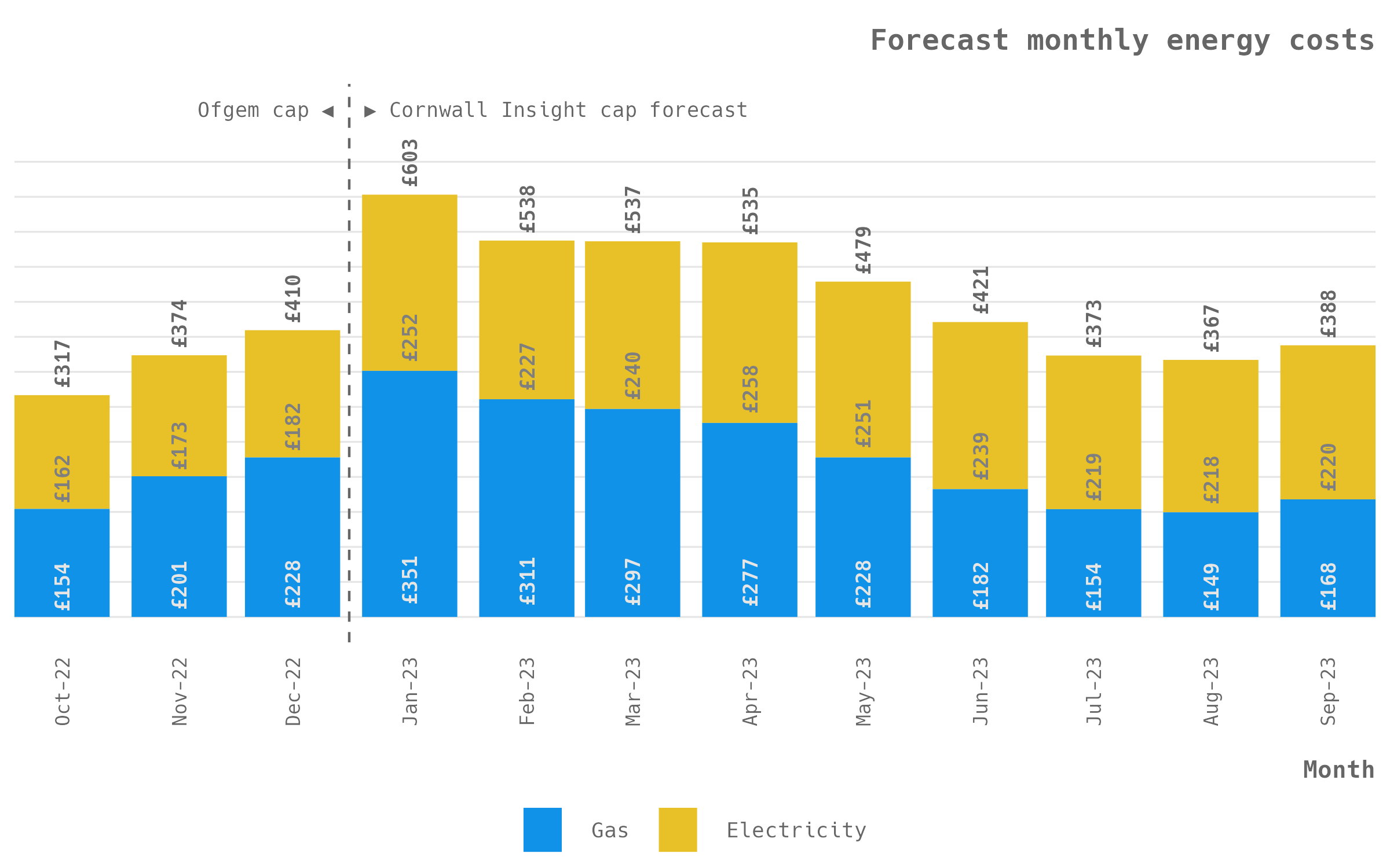
Estimated monthly costs using Ofgem’s default usage figures
Plot code
default_costs_plot <- ggplot(cost_simulator,
                             aes(x = ref_month, y = default_cost, fill = fuel)) +
  geom_col() +
  geom_text(
    mapping = aes(y = default_cost, colour = fuel,
                  label = scales::dollar(default_cost, prefix = "£", accuracy = 1)),
    position = position_stack(vjust = 0.05),
    size = 3,
    angle = 90,
    hjust = 0,
    family = "Hack",
    fontface = "bold",
    show.legend = FALSE
  ) +
  geom_text(
    data = month_totals,
    mapping = aes(y = total, x = ref_month,
                  label = scales::dollar(total, prefix = "£", accuracy = 1)),
    inherit.aes = FALSE,
    size = 3,
    angle = 90,
    hjust = 0,
    nudge_y = 10,
    family = "Hack",
    colour = "grey40",
    fontface = "bold"
  ) +
  geom_vline(xintercept = as.Date("2022-12-16"), colour = "grey40",
             linetype = "dashed") +
  annotate(
    geom = "text", x = as.Date("2022-12-12"), y = 725,
    label = "Ofgem cap ︎◀︎", size = 3,
    family = "Hack", colour = "grey40", hjust = 1
  ) +
  annotate(
    geom = "text", x = as.Date("2022-12-20"), y = 725,
    label = "▶︎ Cornwall Insight forecast", size = 3,
    family = "Hack", colour = "grey40", hjust = 0
  ) +
  scale_y_continuous(limits = c(0, 725), breaks = seq(0, 650, 50)) +
  scale_x_date(date_labels = "%b-%y", date_breaks = "1 month",
               expand = expansion()) +
  scale_fill_manual(values = energy_colours, labels = c("Electricity", "Gas")) +
  scale_colour_manual(values = c("electricity" = "grey50", "gas" = "grey90")) +
  labs(
    title = "Forecast monthly energy costs",
    x = "Month",
  ) +
  mattR::theme_lpsdgeog() +
  theme(
    panel.grid.minor = element_blank(),
    panel.grid.major.x = element_blank(),
    axis.text.x = element_text(angle = 90),
    axis.text.y = element_blank(),
    axis.title.y = element_blank(),
    legend.position = "bottom",
    legend.title = element_blank()
  )
What’s it going to cost me?
So given that I know my annual consumption for gas and electricity I can replace the Ofgem figures with my own. In the cost_simulator code, let’s switch out the 3,100 kWh for electricity with the 2,200 kWh I use and the 12,000 kWh for gas with the 8,200 kWh I use, and I’m looking an estimated annual cost of £3,719.
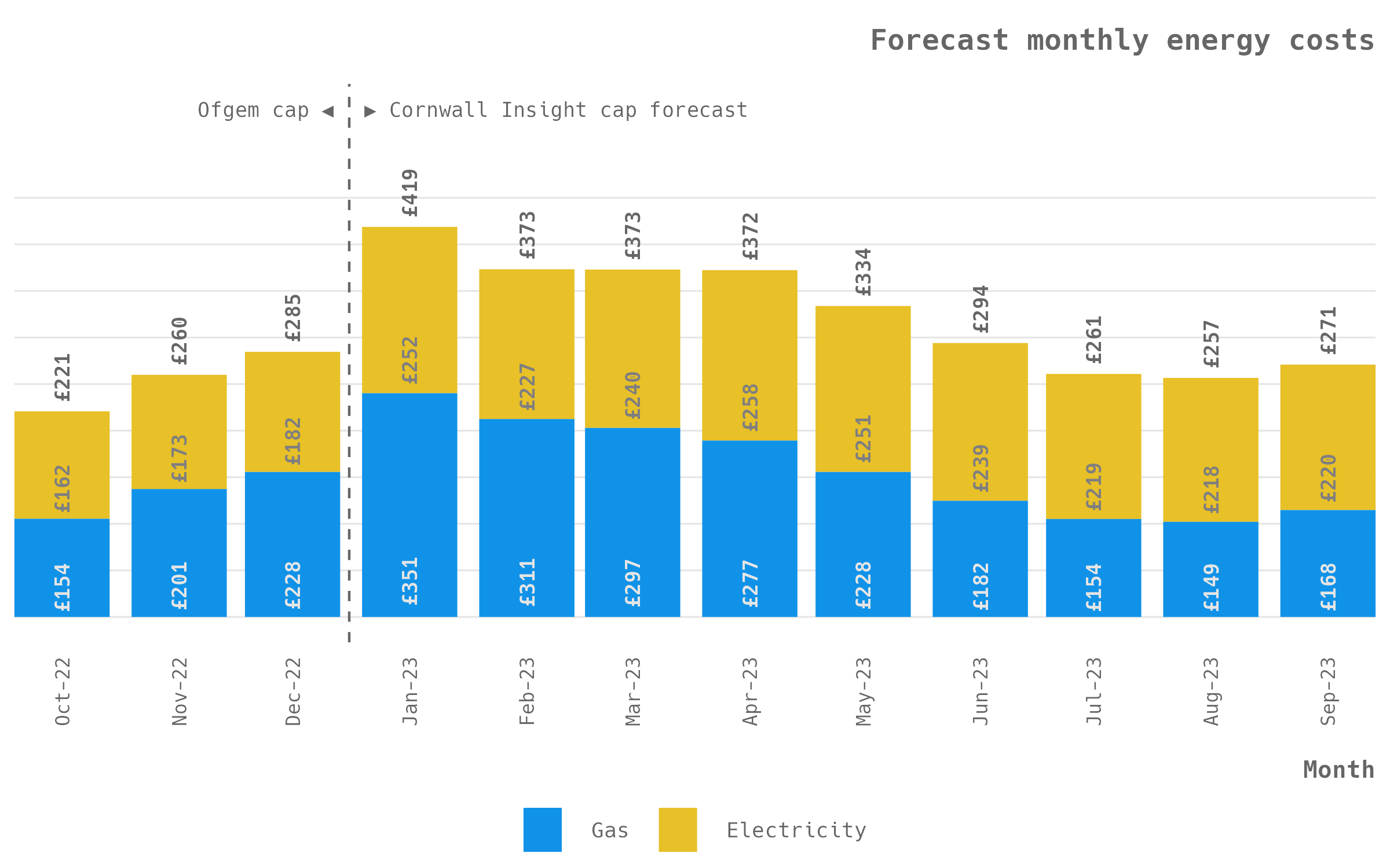
My estimated monthly energy costs
Does it feel right? I don’t know. Personally, I think that my gas usage is actually more sharp than the pattern from the UK total. I live in a two adult household, so in summer months besides each of use having a shower each day and doing the washing up. We live in a ground floor Victorian era flat, while it has double glazing it remains a very draughty property, I doubt it has much insulation, and exposed floorboards are hardly helping, and it rarely feels toasty at the best of times.
If we look at our analysis of Energy Trends we can see that the months of October to March account for around 54% of electricity use and 64% of gas use. But I wouldn’t be surprised if my total is nearer to 80% of my total gas consumption.
> energy_trend_summary |>
    filter(month > 9 | month < 4) |>
    group_by(fuel) |>
    summarise(prop = sum(prop))

# A tibble: 2 × 2
  fuel         prop
  <chr>       <dbl>
1 electricity 0.539
2 gas         0.642
Despite the fact that I might have a more extreme variation in my monthly gas consumption than the UK average, it’s probably still better than taking my annual consumption and usage dividing it into 12 equal chunks and applying the estimated cap prices. Which we can also simulate.
flat_assumption <- cap_estimates |>
  mutate(
    default_elec = electricity * 3100/12,
    default_gas = gas * 12000/12,
    default_total = default_elec + default_gas,
    my_elec = electricity * 2200/12,
    my_gas = gas * 8200/12,
    my_total = my_elec + my_gas
  ) |>
  select(month, starts_with("default"), starts_with("my"))
> flat_assumption
# A tibble: 12 × 7
   month default_elec default_gas default_total my_elec my_gas my_total
   <int>        <dbl>       <dbl>         <dbl>   <dbl>  <dbl>    <dbl>
 1    10         162.        165.          327.    115.   113.     228.
 2    11         162.        165.          327.    115.   113.     228.
 3    12         162.        165.          327.    115.   113.     228.
 4     1         219.        230.          449.    155.   157.     313.
 5     2         219.        230.          449.    155.   157.     313.
 6     3         219.        230.          449.    155.   157.     313.
 7     4         268.        283.          551.    191.   193.     384.
 8     5         268.        283.          551.    191.   193.     384.
 9     6         268.        283.          551.    191.   193.     384.
10     7         239.        252.          491.    170.   172.     342.
11     8         239.        252.          491.    170.   172.     342.
12     9         239.        252.          491.    170.   172.     342.

> round(sum(flat_assumption$default_total))
[1] 5456

> round(sum(flat_assumption$my_total))
[1] 3799
The annual figures aren’t substantially changed, around £80 for my consumption and £120 for the Ofgem default consumption, but the monthly estimates are notably different. Some of this is probably a function of the steep jump predicted for the cap from January. However, these figures are substantially above the prices than the previous price caps or energy prices people have been used to paying. Until last October when my last fixed term contract ended, I was paying just £68 per month for gas and electricity!
What’s it going to cost you?
Given that I’ve built this relatively simple simulator it shouldn’t be too difficult to make it into something that others can use. So that’s what I’ve done, you can access it here.
It was also a great opportunity to try out using Quarto, the successor to RMarkdown, but I’ll save that for another post.
-
“Cap” is probably the wrong term here, it does not limit the total cost a customer can be charged, rather it places a maximum on the amount that can be charged per unit of energy. ↩︎
-
I’m no longer a government employee so I’m finally able to publicly rant about things. ↩︎
-
Though given the experience with Covid, where the government regularly delayed taking action or as little as possible to satisfy its various noisy fringes and vested interests, I’m not that surprised. ↩︎
-
I’m not scraping an inordinately large number of PDFs again. ↩︎
-
Or at least if they do it’s not very easy to locate. ↩︎
-
Each “table” here is an Excel spreadsheet that contains within it several tabs with separate tables, but what we’re after is the monthly x-watt-hour figures (gas is in gigawatt-hours, electricity in terawatt-hours, gas is also available in million cubic metres but converting that to watt-hours is messy and BEIS have already done that). ↩︎